实验设计与分析(第6版,Montgomery)第3章单因子实验:方差分析3.11思考题3.1 R语言解题
本文是实验设计与分析(第6版,Montgomery著,傅珏生译) 第3章单因子实验:方差分析3.11思考题3.1 R语言解题。主要涉及单因子方差分析,正态性假设检验,残差与拟合值的关系图,散点图,LSD法。
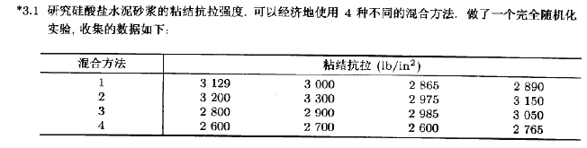
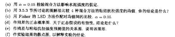
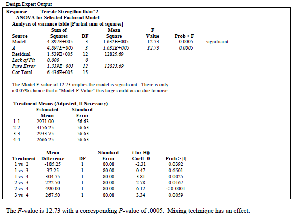
(a) Test the hypothesis that mixing techniques affect the strength of the cement. Use α = 0.05.
X<-c(3129,3000,2865,2890,3200,3300,2975,3150,2800,2900,2985,3050,2600,2700,2600,2765)
A<-factor(rep(1:4, each=4))
miscellany<-data.frame(X,A)
aov.mis<-aov(X~A, data=miscellany)
summary(aov.mis)
> summary(aov.mis)
Df Sum Sq Mean Sq F value Pr(>F)
A 3 489740 163247 12.73 0.000489 ***
Residuals 12 153908 12826
---
Signif. codes:
0 ‘***’ 0.001 ‘**’ 0.01 ‘*’ 0.05 ‘.’ 0.1 ‘ ’ 1
The F-value is 12.73 with a corresponding P-value of .0005. Mixing technique has an effect.
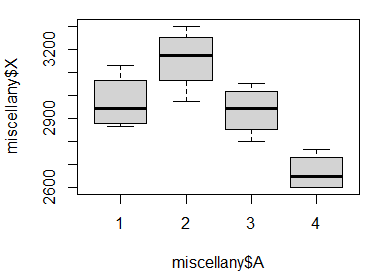
plot(miscellany$X~miscellany$A)
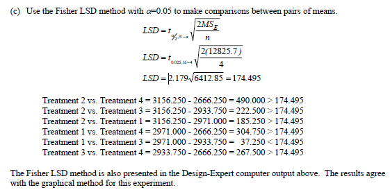
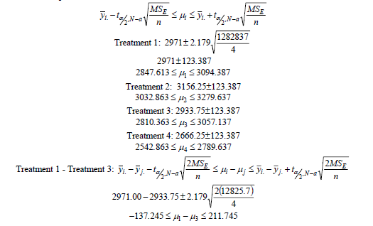
(c) Use the Fisher LSD method with α=0.05 to make comparisons between pairs of means.
install.packages("DescTools")
library(DescTools)
PostHocTest(aov.mis,method = "lsd")
> PostHocTest(aov.mis,method = "lsd")
Posthoc multiple comparisons of means : Fisher LSD
95% family-wise confidence level
$A
diff lwr.ci upr.ci pval
2-1 185.25 10.77016 359.72984 0.0392 *
3-1 -37.25 -211.72984 137.22984 0.6501
4-1 -304.75 -479.22984 -130.27016 0.0025 **
3-2 -222.50 -396.97984 -48.02016 0.0167 *
4-2 -490.00 -664.47984 -315.52016 5.2e-05 ***
4-3 -267.50 -441.97984 -93.02016 0.0059 **
---
Signif. codes: 0 '***' 0.001 '**' 0.01 '*' 0.05 '.' 0.1 ' ' 1
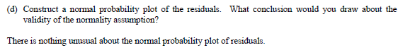
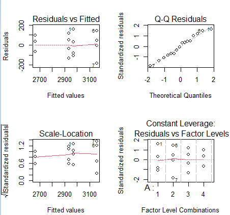
opar <- par(mfrow=c(2,2),cex=.8)
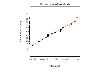
plot(aov.mis)
par(opar)

opar <- par(mfrow=c(2,2),cex=.8)
plot(aov.mis)
par(opar)
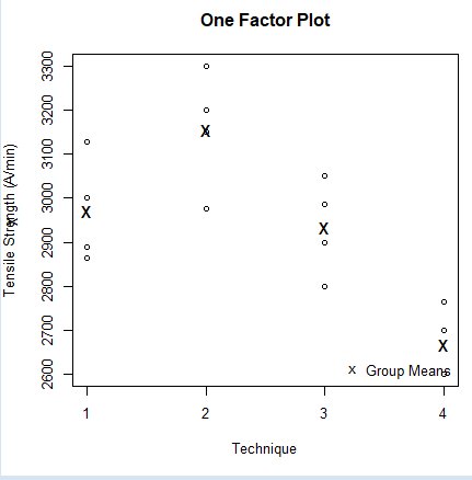
> grp.means <- with(miscellany, tapply(X,A, mean))
> grp.means
1 2 3 4
2971.00 3156.25 2933.75 2666.25
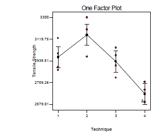
with(miscellany, stripchart (X~A, vert=T,method="overplot" ,pch=1))
stripchart(as.numeric(grp.means) ~as.numeric(names(grp.means)) ,pch="x",cex=1.5,vert=T,add=T)
title(main="One Factor Plot" ,ylab=expression(paste("Tensile Strength (",ring(A),"/min)")) ,xlab="Technique")
legend("bottomright" , "Group Means" ,pch="x" ,bty="n")


install.packages("DescTools")
library(DescTools)
PostHocTest(aov.mis,method = "lsd")
> PostHocTest(aov.mis,method = "lsd")
Posthoc multiple comparisons of means : Fisher LSD
95% family-wise confidence level
$A
diff lwr.ci upr.ci pval
2-1 185.25 10.77016 359.72984 0.0392 *
3-1 -37.25 -211.72984 137.22984 0.6501
4-1 -304.75 -479.22984 -130.27016 0.0025 **
3-2 -222.50 -396.97984 -48.02016 0.0167 *
4-2 -490.00 -664.47984 -315.52016 5.2e-05 ***
4-3 -267.50 -441.97984 -93.02016 0.0059 **
---
Signif. codes: 0 '***' 0.001 '**' 0.01 '*' 0.05 '.' 0.1 ' ' 1
> TukeyHSD(aov.mis)
Tukey multiple comparisons of means
95% family-wise confidence level
Fit: aov(formula = X ~ A, data = miscellany)
$A
diff lwr upr p adj
2-1 185.25 -52.50029 423.00029 0.1493561
3-1 -37.25 -275.00029 200.50029 0.9652776
4-1 -304.75 -542.50029 -66.99971 0.0115923
3-2 -222.50 -460.25029 15.25029 0.0693027
4-2 -490.00 -727.75029 -252.24971 0.0002622
4-3 -267.50 -505.25029 -29.74971 0.0261838
3-2
3-3
3-4
#plot(TukeyHSD(aov.mis) ,las=1)