当前位置：首页 > news >正文

2025最新智能优化算法：野燕麦优化算法（Animated Oat Optimization Algorithm, AOO），MATLAB代码

news 来源：原创 2025/5/26 6:24:18

野燕麦优化算法（Animated Oat Optimization Algorithm, AOO）是2025年提出一种新型元启发式优化算法，其灵感源于自然界中野燕麦种子独特的传播行为。野燕麦是一种一年生草本植物，隶属于禾本科和燕麦属，其种子具有吸湿性和较长的休眠期，能耐受恶劣环境。

该算法精准模拟了野麦种子的三种典型传播机制，具体如下：

三种传播机制

自然扩散：部分不实野燕麦种子从植物上脱落后，借助风、水或动物等自然因素进行传播。这种传播模式具有显著随机性，可在广泛的解空间中进行探索，为算法的全局搜索能力奠定基础。
吸湿滚动：不实野燕麦种子在吸湿运动影响下，其主芒会发生扭曲与旋转，进而驱动整个种子滚动传播。此过程可使种子在无障碍物的区域高效移动，扩大搜索范围，增强算法的局部开发能力
遇阻推进：当种子在滚动传播过程中遇到障碍物时，会储存能量，并在满足特定条件时触发推进机制，实现进一步扩散。这一特性有助于算法在复杂环境中跳脱局部最优解，提升全局优化性能

算法优势及应用

AOO算法的核心机制聚焦于 “种子分布 — 能量积蓄 — 滚动推进” 的耦合搜索策略，其数学建模巧妙地平衡了解空间中的探索与开发能力，确保了算法在解空间中的强探索能力与稳定收敛性能。在实际应用中，AOO算法展现出了显著优势，成功解决了诸多复杂优化问题，尤其在无线传感网络节点定位及工程设计优化等实际应用场景中具有广阔的应用前景

部分MATLAB代码：

clc
clear
close all
% Number of search agents (population size in optimization algorithms)
SearchAgents_no = 30;  
% Dimension of the problem (number of decision variables)
dim = 20;  
% Objective function: 'cec22_func' (CEC 2022 benchmark function)
fhd = str2func('cec22_func');  
% Function number (specific benchmark function in CEC 2022 suite)
Fnum = 12;  
% Maximum number of iterations (stopping condition)
Max_iteration = 1000;  
% Lower bound of the search space (for each variable)
lb = -100;  
% Upper bound of the search space (for each variable)
ub = 100;  
%% optimization algorithm
for i = 1:12
Function_name = i;
[Best_score,Best_pos,cg_curve,search_history,ave_fit,x_1st] = AOOv4(fhd,dim,SearchAgents_no,Max_iteration,lb,ub,Function_name);
Best_score
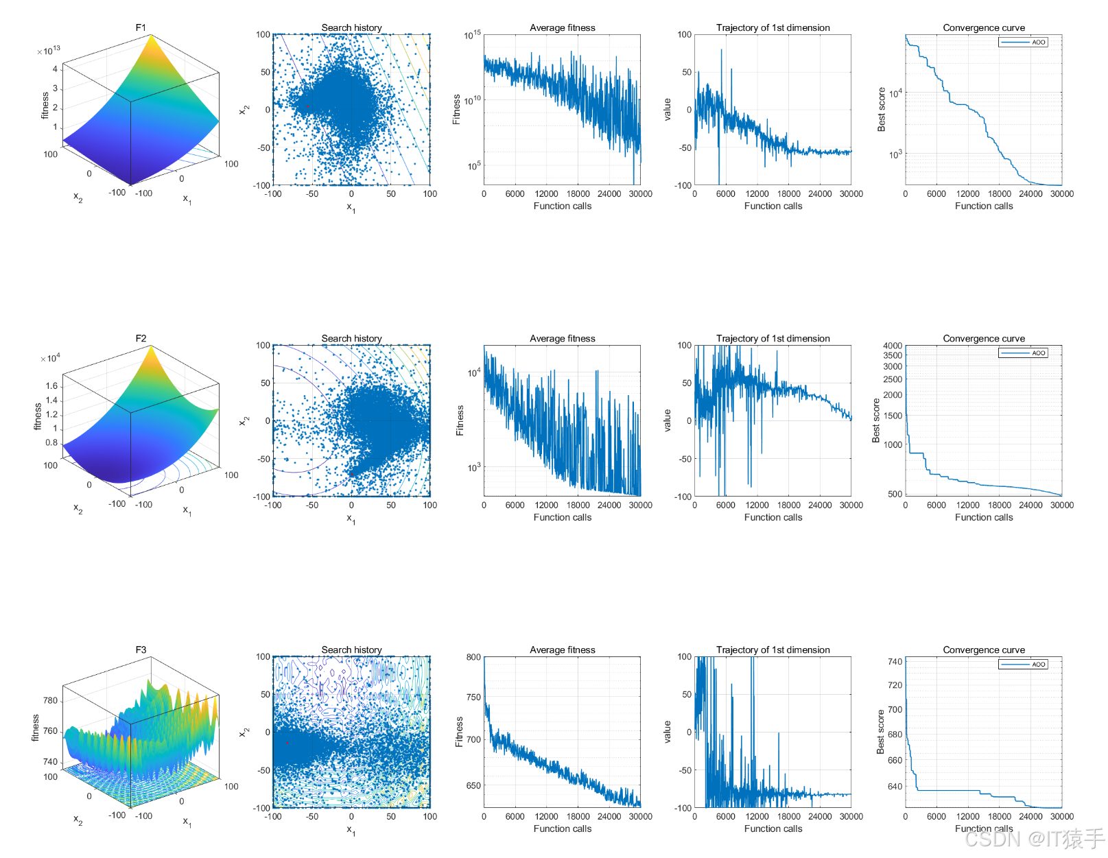
%% plot
figure(i);
set(gcf, 'Position', [150, 350, 1500, 300]);
subplot_width = 1500 / 5;  
subplot_height = 300 / 1;   
padding = 0.05;  
effective_width = (1 - padding * 4) / 5.5;
effective_height = 0.7 ;
left_positions = 0.04 + (0:4) * (effective_width + padding);
adjustedColormap = parula;
colormap(adjustedColormap);
subplot('Position', [left_positions(1), padding*3, effective_width, effective_height]);
func_plot(Function_name);
title(strcat('F', num2str(Function_name)));
xlabel('x_1');
ylabel('x_2');
zlabel('fitness');
set(gca, 'Box', 'on', 'BoxStyle', 'full', 'LineWidth', 0.25);
view(3);
grid on;
% search history
subplot('Position', [left_positions(2), padding*3, effective_width, effective_height]);
grid off;
func_plot_2(Function_name);
hold on;
scatter(search_history(:,1), search_history(:,2), '.');
hold on;
scatter(Best_pos(:,1), Best_pos(:,2), 'r.');
title('Search history');
xlabel('x_1');
ylabel('x_2');
xlim([lb, ub]);
ylim([lb, ub]);
set(gca, 'color', 'none');
grid on;
% average fitness
subplot('Position', [left_positions(3), padding*3, effective_width, effective_height]);
semilogy(ave_fit, 'Linewidth', 1);
grid on;
title('Average fitness');
xlabel('Function calls');
ylabel('Fitness');
xlim([0, Max_iteration ]);
set(gca, 'XTickLabel', arrayfun(@(x) num2str(x), 0:6000:30000, 'UniformOutput', false), 'FontAngle', 'normal');
% Trajectory of 1st dimension
subplot('Position', [left_positions(4), padding*3, effective_width, effective_height]);
plot(x_1st(:,1), 'Linewidth', 1);
title('Trajectory of 1st dimension');
grid on;
xlabel('Function calls');
ylabel('value');
xlim([0, Max_iteration]);
set(gca, 'XTickLabel', arrayfun(@(x) num2str(x), 0:6000:30000, 'UniformOutput', false), 'FontAngle', 'normal');
% 收敛曲线图
subplot('Position', [left_positions(5), padding*3, effective_width, effective_height]);
semilogy(cg_curve, 'Linewidth', 1);
title('Convergence curve');
xlabel('Function calls');
ylabel('Best score');
axis tight;
grid on;
box on;
legend('AOO', 'fontsize', 6, 'location', 'best');
set(gca, 'color', 'none');
xlim([0, Max_iteration]);
set(gca, 'XTickLabel', arrayfun(@(x) num2str(x), 0:6000:30000, 'UniformOutput', false), 'FontAngle', 'normal');
saveas(gcf, sprintf('F%d.eps', Function_name), 'epsc'); % 保存为 EPS
saveas(gcf, sprintf('F%d.svg', Function_name), 'svg');  % 保存为 SVG
Dive_Explor_Exploit(SearchAgents_no,Max_iteration,dim,Function_name,search_history)
end

部分结果