当前位置：首页 > news >正文

基于文本挖掘与情感分析的B站《唐探1900》弹幕研究

news 来源：原创 2025/5/26 5:54:41

1.项目背景

着数字媒体平台的快速发展和用户参与度的不断提升，弹幕作为新兴的实时互动媒介逐渐成为网络视频文化研究和用户行为分析领域关注的重点，弹幕数据作为反映观众真实观影体验和情感态度的重要载体之一，其蕴含的用户行为模式和情感变化轨迹备受关注。通过对弹幕文本数据的系统挖掘和情感分析，不仅有助于揭示不同时间维度下观众的参与特征和内容偏好，还能为影视内容优化、用户运营策略和观影文化研究提供数据支持。该项目以《唐探1900》电影在B站的52,780条弹幕数据为基础，围绕弹幕的时间分布特征、用户活跃度差异、高频词汇分析及情感变化趋势，开展文本挖掘、情感分析和可视化研究，旨在为数字时代的观影行为理解和平台运营决策提供科学依据。

2.数据说明

字段	说明
弹幕内容	观众发送的弹幕文本
视频时间点	弹幕出现时对应的视频时间（秒）
发送时间	弹幕发送的实际时间（时间戳）
用户标识	发送弹幕的用户唯一标识（已脱敏）

3.Python库导入及数据读取

!pip install snownlp -i https://pypi.tuna.tsinghua.edu.cn/simple/

Looking in indexes: https://pypi.tuna.tsinghua.edu.cn/simple/
Requirement already satisfied: snownlp in /opt/conda/lib/python3.11/site-packages (0.12.3)

)

import pandas as pd
import numpy as np
import matplotlib.pyplot as plt
import seaborn as sns
import jieba
from wordcloud import WordCloud
from snownlp import SnowNLP
from collections import Counter, defaultdict
import re

data = pd.read_excel('/home/mw/input/data3813/《唐探1900》的弹幕.xlsx')

4.数据预览及预处理

data.head()

	弹幕内容	视频时间点	发送时间	用户标识
0	观前提醒：第一次看为确保破案体验请屏蔽：凶手，难猜	0:00	2025-05-01 03:07:19	dfbe278
1	炫酷	0:00	2025-05-02 01:59:27	bccc5419
2	来了来了！终于等到！！[给心心]	0:00	2025-04-30 10:28:03	4af8dd7b
3	啊？	0:00	2025-04-30 10:10:39	64b578f3
4	来了	0:00	2025-05-04 06:39:00	6fdf16cf

print('查看数据信息:')
data.info()

查看数据信息:
<class 'pandas.core.frame.DataFrame'>
RangeIndex: 52780 entries, 0 to 52779
Data columns (total 4 columns):#   Column  Non-Null Count  Dtype 
---  ------  --------------  ----- 0   弹幕内容    52780 non-null  object1   视频时间点   52780 non-null  object2   发送时间    52780 non-null  object3   用户标识    52780 non-null  object
dtypes: object(4)
memory usage: 1.6+ MB

print(f'查看重复值:{data.duplicated().sum()}')

查看重复值:0

# 总弹幕数、用户数、时间范围
print('总弹幕数:', len(data))
print('用户数:', data['用户标识'].nunique())
print('时间范围:', data['发送时间'].min(), '至', data['发送时间'].max())

总弹幕数: 52780
用户数: 27193
时间范围: 2025-04-30 10:00:24 至 2025-05-21 09:55:29

把发送时间转为date格式，然后提取里面的发送日期和发送的时间，为后续用户分析做准备，然后把视频时间节点转为分钟数。

# 发送时间拆分为日期和小时
data['发送时间'] = pd.to_datetime(data['发送时间'], errors='coerce')
data['发送日期'] = data['发送时间'].dt.date
data['发送小时'] = data['发送时间'].dt.hour# 视频时间点（格式为 mm:ss）转为分钟数
def mmss_to_minute(t):try:m, s = t.split(':')return int(m)except:return Nonedata['视频时间点'] = data['视频时间点'].apply(mmss_to_minute)

再针对弹幕内容进行分词处理，这里使用的是jieba库，加上一些适合这部电影的分词。

jieba.load_userdict('movie_userdict.txt')
# 读取停用词表到集合
with open('/home/mw/project/停用词汇总.txt', encoding='utf-8') as f:stopwords = set([line.strip() for line in f if line.strip()])

Building prefix dict from the default dictionary ...
Loading model from cache /tmp/jieba.cache
Loading model cost 0.885 seconds.
Prefix dict has been built successfully.

def cut_and_filter(text):# jieba.lcut返回分词列表words = jieba.lcut(str(text))# 过滤停用词和空白return [w for w in words if w not in stopwords and w.strip()]# 新增一列“分词结果”
data['分词'] = data['弹幕内容'].apply(cut_and_filter)# 预览前几行
data[['弹幕内容', '分词']].head()

	弹幕内容	分词
0	观前提醒：第一次看为确保破案体验请屏蔽：凶手，难猜	[观前, 提醒, 第一次, 看为, 确保, 破案, 体验, 屏蔽, 凶手]
1	炫酷	[炫酷]
2	来了来了！终于等到！！[给心心]	[来了, 来了, 心心]
3	啊？	[]
4	来了	[来了]

data = data[['弹幕内容','分词', '视频时间点', '发送日期', '发送小时','用户标识']]
data.head()

	弹幕内容	分词	发送日期	发送小时	用户标识
0	观前提醒：第一次看为确保破案体验请屏蔽：凶手，难猜	[观前, 提醒, 第一次, 看为, 确保, 破案, 体验, 屏蔽, 凶手]	2025-05-01	3	dfbe278
1	炫酷	[炫酷]	2025-05-02	1	bccc5419
2	来了来了！终于等到！！[给心心]	[来了, 来了, 心心]	2025-04-30	10	4af8dd7b
3	啊？	[]	2025-04-30	10	64b578f3
4	来了	[来了]	2025-05-04	6	6fdf16cf

5.可视化分析

5.1弹幕在视频时间轴上的分布

plt.figure(figsize=(12, 4))
# 使用有效的bins数量，避免太多空桶
time_min = data['视频时间点'].min()
time_max = data['视频时间点'].max()
bins = min(int(time_max - time_min + 1), 140)  # 限制最大bins数为140plt.hist(data['视频时间点'], bins=bins, alpha=0.7, color='skyblue', edgecolor='black')
plt.xlabel('视频时间点（分钟）')
plt.ylabel('弹幕数量')
plt.title('弹幕在视频时间轴上的分布')
plt.xlim(time_min, time_max)  # 设置x轴范围从最小值到最大值
plt.grid(axis='y', linestyle='--', alpha=0.7)
plt.tight_layout()
plt.show()

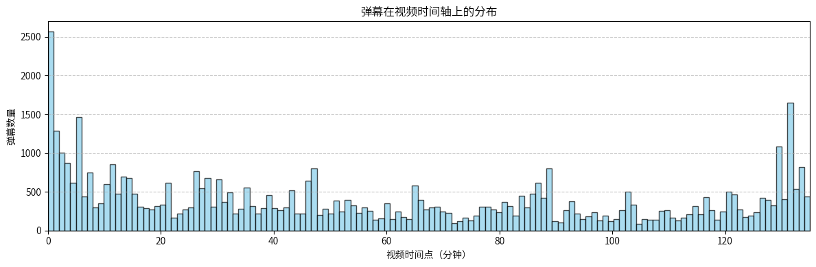
弹幕高度集中在电影开头（0-5分钟）和结尾（120-130分钟），呈现典型的"首尾热"现象。开头弹幕可能是观众的期待情绪和问候，结尾弹幕则是对剧情结局、彩蛋的讨论，中间段弹幕相对平稳，但在某些时间点（如45分钟左右）有小高峰，可能对应剧情转折点。

5.2每天弹幕数量分布

# 按日期分组并计数
daily_counts = data.groupby('发送日期').size()plt.figure(figsize=(12, 4))
plt.plot(daily_counts.index, daily_counts.values, marker='o', linestyle='-', color='#1f77b4')
plt.xlabel('日期')
plt.ylabel('弹幕数量')
plt.title('每日弹幕数量分布')
plt.xticks(daily_counts.index[::2], rotation=0)  # 每隔2个日期显示一个刻度，避免拥挤
plt.grid(axis='y', linestyle='--', alpha=0.7)
plt.tight_layout()
plt.show()

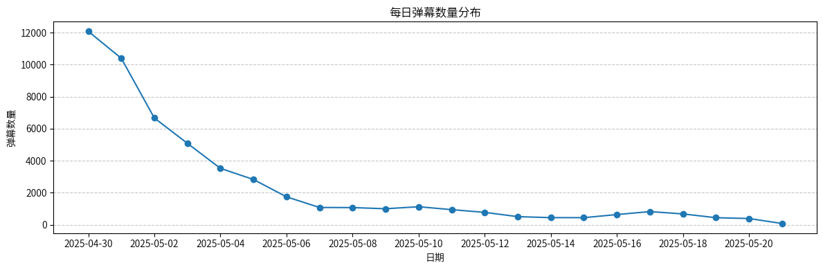
弹幕数量呈现明显的衰减趋势，从首日的12000+条急剧下降到后期的几百条。这符合电影热度的自然衰减规律，首日观影人数最多，随着时间推移关注度逐渐降低。影片是4月30日在B站发布的，4月30日-5月3日是弹幕的黄金期。

5.3每小时弹幕活跃度分布

hourly_counts = data.groupby('发送小时').size()plt.figure(figsize=(12, 4))
bars = plt.bar(hourly_counts.index, hourly_counts.values, color='skyblue', edgecolor='black', alpha=0.8)# 在柱状图顶部添加数值标签
for bar in bars:height = bar.get_height()plt.text(bar.get_x() + bar.get_width()/2., height + 100,f'{int(height)}', ha='center', va='bottom', fontsize=8)plt.xlabel('小时')
plt.ylabel('弹幕数量')
plt.title('每小时弹幕活跃度分布')
plt.xticks(range(0, 24), rotation=0)  # 确保显示所有24小时
plt.grid(axis='y', linestyle='--', alpha=0.7)
plt.tight_layout()
plt.show()

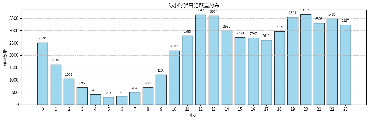
弹幕活跃度呈现典型的双峰分布：

晚间高峰（19-22点）：3500+条，是观影黄金时段
午间小高峰（12-13点）：3600+条，可能是午休时间观影
凌晨低谷（3-8点）：最低不足500条
符合用户作息规律，晚上是主要的娱乐时间

5.4用户活跃度分析

user_counts = data['用户标识'].value_counts()
top20_users = user_counts.head(20)plt.figure(figsize=(12, 4))
bars = plt.bar(range(len(top20_users)), top20_users.values, color='skyblue', edgecolor='black', alpha=0.8)# 在柱状图顶部添加数值标签
for bar in bars:height = bar.get_height()plt.text(bar.get_x() + bar.get_width()/2., height + 5,f'{int(height)}', ha='center', va='bottom', fontsize=8, rotation=0)plt.xlabel('用户标识')
plt.ylabel('弹幕数')
plt.title('最活跃用户Top20')
# 保留原始用户标识，旋转90度显示
plt.xticks(range(len(top20_users)), top20_users.index, rotation=90)
plt.grid(axis='y', linestyle='--', alpha=0.7)
plt.tight_layout()
plt.show()

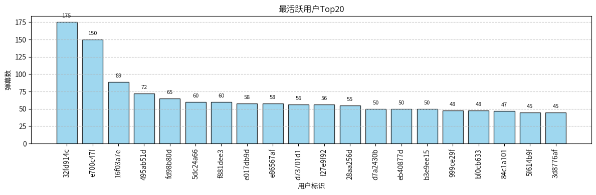
用户参与度存在明显的长尾分布，最活跃用户发送178条弹幕，而第20名仅45条。前两名用户（178条、150条）显著高于其他用户，可能是电影的忠实粉丝。

5.5高频词分析

# 合并所有分词为一个列表
all_words = [word for words in data['分词'] for word in words]
word_freq = Counter(all_words)font_path = '/home/mw/project/SIMHEI.TTF' wc = WordCloud(font_path=font_path,background_color='white',width=800,height=400,max_words=200
)wc.generate_from_frequencies(word_freq)
plt.figure(figsize=(15, 7))
plt.imshow(wc, interpolation='bilinear')
plt.axis('off')
plt.title('《唐探1900》弹幕高频词云', fontsize=20)
plt.show()

弹幕内容体现了观众的多元化关注点：

演员关注：刘昊然、王宝强等主演名字突出
情感表达：哈哈哈、好看、经典等正面评价占主导
剧情讨论：推理、侦探、电影等核心元素
网络文化：666、doge等B站特色弹幕文化
节日氛围：影片上映B站的时候，正好是4月30日，接近五一假期，所以许多人都在发五一快乐。

6.情感分析

6.1SnowNLP

SnowNLP是一个专门为中文文本处理设计的Python自然语言处理库，由韩寒开发。它提供了中文分词、词性标注、情感分析、关键词提取、文本摘要等功能，特别适合处理中文社交媒体文本。

SnowNLP的情感分析基于机器学习方法，主要特点包括：

训练数据: 使用大量中文商品评论数据进行训练
算法基础: 基于朴素贝叶斯分类器
输出格式: 返回0-1之间的连续值，越接近1表示越积极，越接近0表示越消极
中性判断: 0.5为中性分界点

SnowNLP的优势
✅ 专为中文优化: 对中文语法和表达习惯有很好的适应性
✅ 使用简便: API简洁，无需复杂配置
✅ 训练数据丰富: 基于大量真实的中文评论数据
✅ 连续输出: 提供细粒度的情感强度评分

SnowNLP的局限性
❌ 领域适应性: 主要基于商品评论训练，对其他领域可能不够准确
❌ 网络语言: 对新兴网络用语、方言、缩写的识别能力有限
❌ 特定平台: 对B站等特定平台的文化表达缺乏针对性
❌ 更新频率: 词汇库更新相对滞后

考虑到B站弹幕的独特性，本研究采用了SnowNLP + 自定义词典的双重分析策略，词典由claude4.0提供，内容如下：

Image Name

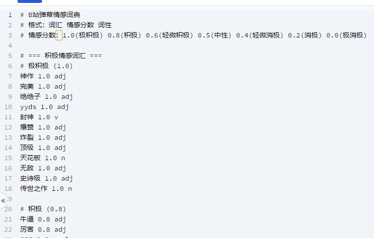
def load_sentiment_dict():sentiment_dict = {}with open('bilibili_sentiment_dict.txt', 'r', encoding='utf-8') as f:for line in f:line = line.strip()if line and not line.startswith('#'):parts = line.split()if len(parts) >= 2:word = parts[0]score = float(parts[1])sentiment_dict[word] = scorereturn sentiment_dict

def analyze_sentiment(text, sentiment_dict):if pd.isna(text) or not str(text).strip():return 0.5, '中性'text = str(text).strip()# 文本预处理text = re.sub(r'[哈]{3,}', '哈哈哈', text)text = re.sub(r'[？]{2,}', '？？', text)text = re.sub(r'[！]{2,}', '！！', text)text = re.sub(r'6{4,}', '6666', text)text = re.sub(r'2{3,}3{3,}', '2333', text)# SnowNLP基础分析s = SnowNLP(text)snownlp_score = s.sentiments# 自定义词典分析custom_score = 0.5sentiment_scores = []# 滑动窗口匹配i = 0while i < len(text):found = Falsefor length in range(min(10, len(text) - i), 0, -1):word = text[i:i+length]if word in sentiment_dict:sentiment_scores.append(sentiment_dict[word])i += lengthfound = Truebreakif not found:i += 1if sentiment_scores:custom_score = np.mean(sentiment_scores)# 加权融合if custom_score != 0.5:base_score = 0.3 * snownlp_score + 0.7 * custom_scoreelse:base_score = snownlp_score# 特殊规则调整score = base_scoreif '？' in text:score = max(0.0, score - 0.1)if '！' in text:if score > 0.5:score = min(1.0, score + 0.1)else:score = max(0.0, score - 0.1)if any(num in text for num in ['666', '6666', '2333', '8888']):score = min(1.0, score + 0.15)if any(word in text for word in ['yyds', 'awsl', 'hhh', '笑死', '爱了', '绝了', '哈哈哈']):score = min(1.0, score + 0.2)if any(word in text for word in ['mmp', 'wtf', '垃圾', '烂片', '傻逼']):score = max(0.0, score - 0.3)if any(neg in text for neg in ['不', '没', '别', '非', '无']):if score > 0.6:score = max(0.3, 1 - score)elif score < 0.4:score = min(0.7, 1 - score)score = np.clip(score, 0.0, 1.0)# 情感分类if score >= 0.6:label = '积极'elif score <= 0.4:label = '消极'else:label = '中性'return score, label

sentiment_dict = load_sentiment_dict()
print(f"词典加载完成：{len(sentiment_dict)}个词汇")

词典加载完成：254个词汇

results = data['弹幕内容'].apply(lambda x: analyze_sentiment(x, sentiment_dict))
data['情感得分'] = results.apply(lambda x: x[0])
data['情感分类'] = results.apply(lambda x: x[1])

sentiment_counts = data['情感分类'].value_counts()
print("情感分布:", dict(sentiment_counts))
print(f"平均得分: {data['情感得分'].mean():.3f}")

情感分布: {'积极': 28557, '中性': 14834, '消极': 9389}
平均得分: 0.618

data.head()

	弹幕内容	分词	发送日期	发送小时	用户标识	情感得分	情感分类
0	观前提醒：第一次看为确保破案体验请屏蔽：凶手，难猜	[观前, 提醒, 第一次, 看为, 确保, 破案, 体验, 屏蔽, 凶手]	2025-05-01	3	dfbe278	0.579422	中性
1	炫酷	[炫酷]	2025-05-02	1	bccc5419	0.948682	积极
2	来了来了！终于等到！！[给心心]	[来了, 来了, 心心]	2025-04-30	10	4af8dd7b	0.801884	积极
3	啊？	[]	2025-04-30	10	64b578f3	0.426233	中性
4	来了	[来了]	2025-05-04	6	6fdf16cf	0.577870	中性

6.2可视化分析

# 创建子图布局 (2行2列，第三个图占2列)
fig = plt.figure(figsize=(15, 10))# 第一个子图：情感分类饼图
ax1 = plt.subplot(2, 2, 1)
sentiment_counts = data['情感分类'].value_counts()
colors = {'积极': '#F08080', '中性': '#87CEEB', '消极': '#90EE90'}  # 积极改成红色，消极改成绿色
pie_colors = [colors.get(label, 'gray') for label in sentiment_counts.index]wedges, texts, autotexts = ax1.pie(sentiment_counts.values, labels=sentiment_counts.index, autopct='%1.1f%%',colors=pie_colors, startangle=90)# 美化饼图文字
for autotext in autotexts:autotext.set_color('white')autotext.set_fontweight('bold')autotext.set_fontsize(11)for text in texts:text.set_fontsize(12)text.set_fontweight('bold')ax1.set_title('情感分类分布', fontsize=14, fontweight='bold', pad=20)# 第二个子图：情感得分分布直方图
ax2 = plt.subplot(2, 2, 2)
n, bins, patches = ax2.hist(data['情感得分'], bins=35, alpha=0.7, edgecolor='black', linewidth=0.5)# 根据得分给直方图着色（颜色对调）
for i, (patch, bin_center) in enumerate(zip(patches, (bins[:-1] + bins[1:]) / 2)):if bin_center <= 0.4:patch.set_facecolor('#90EE90')  # 消极-绿色elif bin_center >= 0.6:patch.set_facecolor('#F08080')  # 积极-红色else:patch.set_facecolor('#87CEEB')  # 中性-蓝色# 添加分界线
ax2.axvline(x=0.5, color='red', linestyle='--', alpha=0.8, linewidth=2, label='中性线(0.5)')
ax2.axvline(x=0.4, color='orange', linestyle=':', alpha=0.7, linewidth=1.5, label='消极阈值(0.4)')
ax2.axvline(x=0.6, color='green', linestyle=':', alpha=0.7, linewidth=1.5, label='积极阈值(0.6)')ax2.set_title('情感得分分布', fontsize=14, fontweight='bold')
ax2.set_xlabel('情感得分', fontsize=11)
ax2.set_ylabel('弹幕数量', fontsize=11)
ax2.legend(fontsize=9)
ax2.grid(True, alpha=0.3)# 第三个子图：时间趋势分析（占2列）
ax3 = plt.subplot(2, 1, 2)  # 第2行，占满整行# 转换视频时间点为分钟
def time_to_minutes(time_str):try:if pd.isna(time_str):return 0time_str = str(time_str).strip()if ':' in time_str:parts = time_str.split(':')if len(parts) == 2:minutes = int(parts[0])seconds = int(parts[1])return minutes + seconds / 60return float(time_str) if str(time_str).replace('.', '').isdigit() else 0except:return 0# 处理时间数据
data['视频分钟'] = data['视频时间点'].apply(time_to_minutes)# 按时间区间统计情感得分和弹幕数量
time_interval = 3  # 3分钟区间
data['时间区间'] = (data['视频分钟'] // time_interval) * time_interval# 计算每个时间区间的平均情感得分和弹幕数量
emotion_time = data.groupby('时间区间').agg({'情感得分': 'mean','弹幕内容': 'count'
}).rename(columns={'弹幕内容': '弹幕数量'})# 创建双Y轴
ax3_twin = ax3.twinx()# 绘制情感得分趋势线
line1 = ax3.plot(emotion_time.index, emotion_time['情感得分'], marker='o', linewidth=3, markersize=6, color='purple', label='平均情感得分', alpha=0.8)# 绘制弹幕数量柱状图
bars = ax3_twin.bar(emotion_time.index, emotion_time['弹幕数量'], width=time_interval*0.8, alpha=0.3, color='skyblue', label='弹幕数量', edgecolor='steelblue', linewidth=0.5)# 添加情感区域填充（颜色对调）
ax3.axhline(y=0.5, color='red', linestyle='--', alpha=0.7, linewidth=1.5, label='中性线')
ax3.fill_between(emotion_time.index, emotion_time['情感得分'], 0.5, where=(emotion_time['情感得分'] >= 0.5), color='red', alpha=0.2, label='积极区域')  # 积极改成红色
ax3.fill_between(emotion_time.index, emotion_time['情感得分'], 0.5, where=(emotion_time['情感得分'] < 0.5), color='green', alpha=0.2, label='消极区域')  # 消极改成绿色# 设置坐标轴
ax3.set_xlabel('视频时间（分钟）', fontsize=12, fontweight='bold')
ax3.set_ylabel('平均情感得分', fontsize=12, fontweight='bold', color='purple')
ax3_twin.set_ylabel('弹幕数量', fontsize=12, fontweight='bold', color='steelblue')# 设置Y轴颜色
ax3.tick_params(axis='y', labelcolor='purple')
ax3_twin.tick_params(axis='y', labelcolor='steelblue')# 设置Y轴范围
ax3.set_ylim(0, 1)
ax3_twin.set_ylim(0, max(emotion_time['弹幕数量']) * 1.1)# 添加图例
lines1, labels1 = ax3.get_legend_handles_labels()
lines2, labels2 = ax3_twin.get_legend_handles_labels()
ax3.legend(lines1 + lines2, labels1 + labels2, loc='upper right', fontsize=10)ax3.set_title('情感随视频时间变化趋势', fontsize=14, fontweight='bold', pad=20)
ax3.grid(True, alpha=0.3)# 找出情感最高点和最低点
max_emotion_time = emotion_time['情感得分'].idxmax()
min_emotion_time = emotion_time['情感得分'].idxmin()
max_emotion_score = emotion_time['情感得分'].max()
min_emotion_score = emotion_time['情感得分'].min()# 智能调整标注位置，避免重合
x_range = emotion_time.index.max() - emotion_time.index.min()
y_range = 1.0  # 情感得分范围是0-1
time_center = (emotion_time.index.max() + emotion_time.index.min()) / 2  # 计算时间轴中点# 为高峰点选择合适的标注位置
if max_emotion_time < time_center:# 如果高峰在前半部分，标注放右边max_text_x = max_emotion_time + x_range * 0.15max_ha = 'left'
else:# 如果高峰在后半部分，标注放左边max_text_x = max_emotion_time - x_range * 0.15max_ha = 'right'# 为低谷点选择合适的标注位置
if min_emotion_time < time_center:# 如果低谷在前半部分，标注放右边min_text_x = min_emotion_time + x_range * 0.15min_ha = 'left'
else:# 如果低谷在后半部分，标注放左边min_text_x = min_emotion_time - x_range * 0.15min_ha = 'right'# 调整Y轴位置，避免与趋势线重合
max_text_y = max_emotion_score + 0.08 if max_emotion_score < 0.8 else max_emotion_score - 0.12
min_text_y = min_emotion_score - 0.08 if min_emotion_score > 0.2 else min_emotion_score + 0.12# 标注关键点（优化位置）
ax3.annotate(f'情感高峰\n{max_emotion_time:.0f}分钟\n得分:{max_emotion_score:.3f}', xy=(max_emotion_time, max_emotion_score), xytext=(max_text_x, max_text_y),arrowprops=dict(arrowstyle='->', color='red', alpha=0.8, lw=1.5),fontsize=9, ha=max_ha, va='center',bbox=dict(boxstyle="round,pad=0.3", facecolor='lightcoral', alpha=0.8, edgecolor='red'))ax3.annotate(f'情感低谷\n{min_emotion_time:.0f}分钟\n得分:{min_emotion_score:.3f}', xy=(min_emotion_time, min_emotion_score), xytext=(min_text_x, min_text_y),arrowprops=dict(arrowstyle='->', color='green', alpha=0.8, lw=1.5),fontsize=9, ha=min_ha, va='center',bbox=dict(boxstyle="round,pad=0.3", facecolor='lightgreen', alpha=0.8, edgecolor='green'))plt.tight_layout()
plt.show()

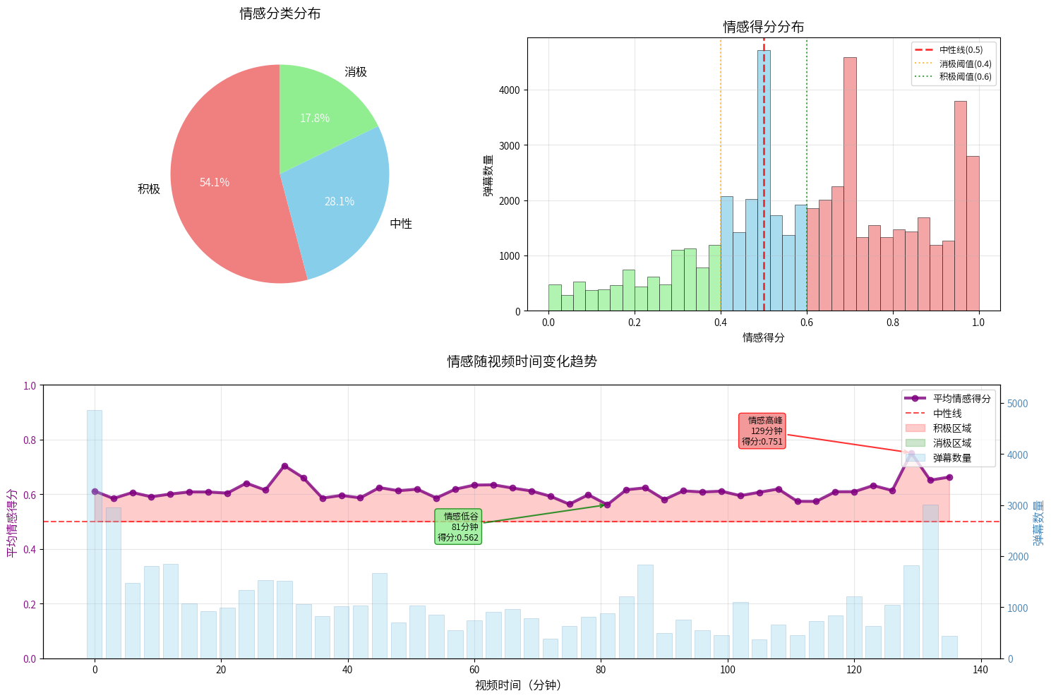
整体情感倾向：从饼图可以看出，观众对《唐探1900》的反应以积极情感为主导，占比54.1%，超过一半。中性情感占28.1%，消极情感仅17.8%。这个比例分布表明电影在观众中的接受度相当不错。
情感得分特征：直方图显示了一个有趣的现象：情感得分呈现明显的右偏分布。大部分弹幕集中在0.5-0.8区间，特别是0.6-0.7区间有个显著峰值。这说明观众的情感反应相对温和积极，很少出现极端的负面或极端的正面评价。
观影过程中的情感波动：情感曲线整体在0.5-0.7之间波动，相对平稳。但有几个值得注意的时间节点：
- 开场阶段（0-10分钟）：弹幕数量很高，但情感相对平稳
- 中段某个时刻（约80分钟附近）：出现了明显的情感低谷，得分降到0.562
- 后半段（约125分钟）：达到情感高峰，得分0.751

总的来说，从数据角度看，这部电影在观众中的表现算是成功的。

7.总结

本项目基于对《唐探1900》弹幕数据的系统分析，得出以下主要结论：

用户参与特征：弹幕分布呈现"首尾热"现象，平均每分钟弹幕量在开头和结尾时段最高，用户活跃度存在显著长尾分布，且呈现明显的时段偏好特征。
内容偏好分析：观众关注的高频词涵盖演员表现（刘昊然、王宝强）和剧情元素（推理、侦探），网络文化表达（666、yyds）与传统观影语言深度融合，体现了B站弹幕文化的独特性。
情感体验量化：通过SnowNLP与自定义词典融合分析，证实观众整体情感倾向积极，积极情感占比54.1%，平均情感得分0.618，情感波动与剧情发展高度吻合，从数据角度来看，这部电影在观众中的表现是成功的。