pvlib(太阳轨迹)
文章目录
- 示例代码
- 分解执行
- 提取太阳轨迹的数据
- 中文参数说明:
- 补充说明:
- 设置坐标系
- 数据处理
- 绘制散点
- 标准化这个颜色块
- 绘制小时的标签
- 标记单个的日期
- 如何讨论针对某个地区日照情况
示例代码
from pvlib import solarposition
import pandas as pd
import numpy as np
import matplotlib.pyplot as plttz = 'Asia/Calcutta'
lat, lon = 28.6, 77.2times = pd.date_range('2019-01-01 00:00:00', '2020-01-01', freq='H', tz=tz)
solpos = solarposition.get_solarposition(times, lat, lon)
# remove nighttime
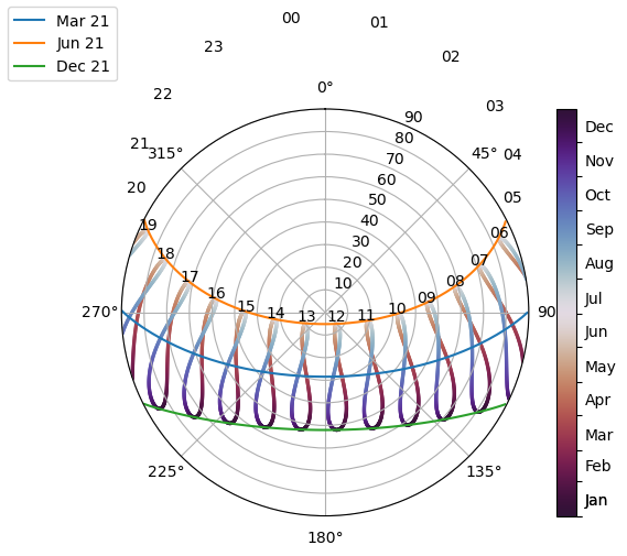
solpos = solpos.loc[solpos['apparent_elevation'] > 0, :]ax = plt.subplot(1, 1, 1, projection='polar')
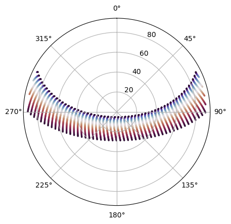
# draw the analemma loops
points = ax.scatter(np.radians(solpos.azimuth), solpos.apparent_zenith,s=2, label=None, c=solpos.index.dayofyear,cmap='twilight_shifted_r')
# add and format colorbar
cbar = ax.figure.colorbar(points)
times_ticks = pd.date_range('2019-01-01', '2020-01-01', freq='MS', tz=tz)
cbar.set_ticks(ticks=times_ticks.dayofyear, labels=[], minor=False)
cbar.set_ticks(ticks=times_ticks.dayofyear+15,labels=times_ticks.strftime('%b'),minor=True)
cbar.ax.tick_params(which='minor', width=0)# draw hour labels
for hour in np.unique(solpos.index.hour):# choose label position by the smallest radius for each hoursubset = solpos.loc[solpos.index.hour == hour, :]r = subset.apparent_zenithpos = solpos.loc[r.idxmin(), :]ax.text(np.radians(pos['azimuth']), pos['apparent_zenith'],str(hour).zfill(2), ha='center', va='bottom')# draw individual days
for date in pd.to_datetime(['2019-03-21', '2019-06-21', '2019-12-21']):times = pd.date_range(date, date+pd.Timedelta('24h'), freq='5min', tz=tz)solpos = solarposition.get_solarposition(times, lat, lon)solpos = solpos.loc[solpos['apparent_elevation'] > 0, :]label = date.strftime('%b %d')ax.plot(np.radians(solpos.azimuth), solpos.apparent_zenith, label=label)ax.figure.legend(loc='upper left')# change coordinates to be like a compass
ax.set_theta_zero_location('N')
ax.set_theta_direction(-1)
ax.set_rmax(90)plt.show()
分解执行
提取太阳轨迹的数据
需要提供时区,经纬度坐标。
from pvlib import solarposition
import pandas as pd
import numpy as np
import matplotlib.pyplot as plttz = 'Asia/Calcutta'
lat, lon = 28.6, 77.2times = pd.date_range('2019-01-01 00:00:00', '2020-01-01', freq='H', tz=tz)
solpos = solarposition.get_solarposition(times, lat, lon)
以下是 solpos 数据前几行的表格示例(包含所有6个参数),并附带中文说明:
| 时间 (IST) | apparent_zenith (°) | zenith (°) | apparent_elevation (°) | elevation (°) | azimuth (°) | equation_of_time (min) |
|---|---|---|---|---|---|---|
| 2019-01-01 00:00:00+05:30 | 172.218 | 172.218 | -2.218 | -2.218 | 180.0 | -3.383 |
| 2019-01-01 01:00:00+05:30 | 167.842 | 167.842 | 2.158 | 2.158 | 185.2 | -3.383 |
| 2019-01-01 02:00:00+05:30 | 158.764 | 158.764 | 11.236 | 11.236 | 193.1 | -3.383 |
| 2019-01-01 03:00:00+05:30 | 144.521 | 144.521 | 25.479 | 25.479 | 203.6 | -3.383 |
| 2019-01-01 04:00:00+05:30 | 124.303 | 124.303 | 45.697 | 45.697 | 217.2 | -3.383 |
| 2019-01-01 05:00:00+05:30 | 97.887 | 97.887 | 72.113 | 72.113 | 233.5 | -3.383 |
| 2019-01-01 06:00:00+05:30 | 80.246 | 80.246 | 89.754 | 89.754 | 246.8 | -3.383 |
| 2019-01-01 07:00:00+05:30 | 70.529 | 70.529 | 99.471 | 99.471 | 257.1 | -3.383 |
中文参数说明:
- apparent_zenith - 表观天顶角(含大气折射修正)
- zenith - 真实天顶角(不含大气折射)
- apparent_elevation - 表观高度角(含大气折射修正,>0可见太阳)
- elevation - 真实高度角(=90°-zenith)
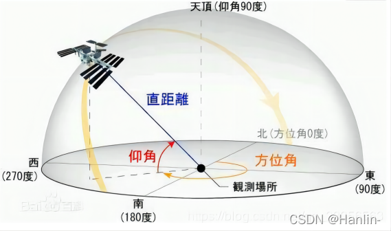
- azimuth - 方位角(正北=0°,顺时针增加,正南=180°)
- equation_of_time - 时差(真太阳时与平太阳时的差值,单位:分钟)
补充说明:
- 夜间时
apparent_zenith≈zenith(大气折射影响可忽略) - 日出/日落时
elevation≈ 0° - 正午时
azimuth≈ 180°(印度位于北半球,太阳在正南方) equation_of_time每日变化极小,因此每小时值相同
关于角度的辨析
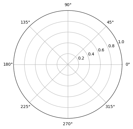
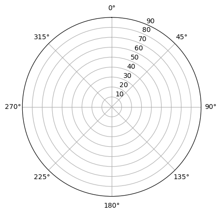
设置坐标系
ax = plt.subplot(1, 1, 1, projection='polar')
ax.set_theta_zero_location('N')# 将极坐标的0度位置设置为北
ax.set_theta_direction(-1)#将极坐标的角度方向设置为顺时针
ax.set_rmax(90)# 把度数转化为0-90
因为是对北半球进行分析的,标准是180度指向正南的方向。
数据处理
表观高度角(apparent_elevation)(含大气折射修正,>0可见太阳)
这个步骤根据这个来去掉黑夜。
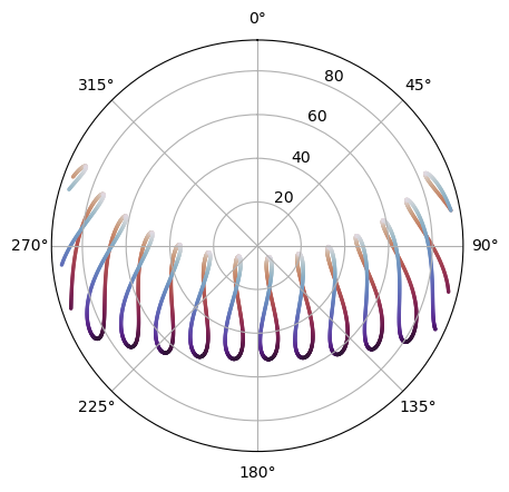
solpos = solpos.loc[solpos['apparent_elevation'] > 0, :]绘制散点
使用 azimuth,apparent_zenith
# draw the analemma loops
points = ax.scatter(np.radians(solpos.azimuth),# X轴:太阳方位角(弧度)solpos.apparent_zenith,   # Y轴:视天顶角(极坐标半径)s=2, label=None, c=solpos.index.dayofyear, # 颜色映射依据:年积日(1-365)cmap='twilight_shifted_r')   # 使用循环色带表示年度周期
如果绘制某个日期的,日线轨迹图。
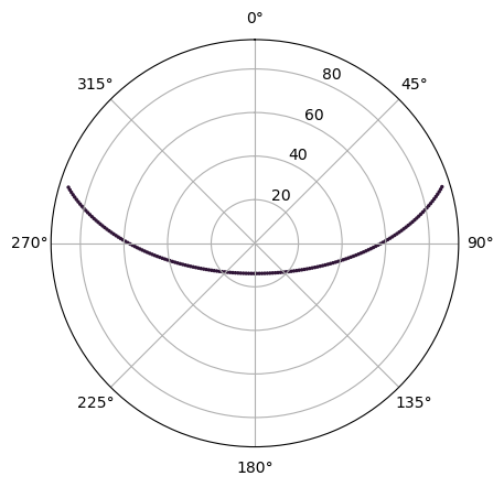
我的理解,这个是强度,因为太阳轨迹,在中间是重合的
对太阳轨迹,使用从春分到夏至的min级别的统计。
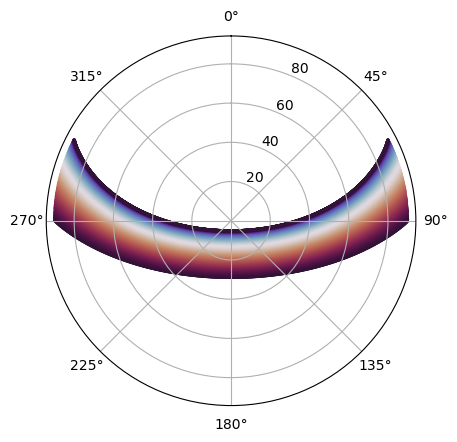
times = pd.date_range('2019-03-20 00:00:00', '2019-06-21 00:00:00', freq='15min', tz=tz)
solpos = solarposition.get_solarposition(times, lat, lon)
标准化这个颜色块
# add and format colorbar
cbar = ax.figure.colorbar(points)
times_ticks = pd.date_range('2019-01-01', '2020-01-01', freq='MS', tz=tz)
cbar.set_ticks(ticks=times_ticks.dayofyear, labels=[], minor=False)
cbar.set_ticks(ticks=times_ticks.dayofyear+15,labels=times_ticks.strftime('%b'),minor=True)
cbar.ax.tick_params(which='minor', width=0)
绘制小时的标签
# draw hour labels
for hour in np.unique(solpos.index.hour):# choose label position by the smallest radius for each hoursubset = solpos.loc[solpos.index.hour == hour, :]r = subset.apparent_zenithpos = solpos.loc[r.idxmin(), :]ax.text(np.radians(pos['azimuth']), pos['apparent_zenith'],str(hour).zfill(2), ha='center', va='bottom')
标记单个的日期
频率设置是5min。
# draw individual days
for date in pd.to_datetime(['2019-03-21', '2019-06-21', '2019-12-21']):times = pd.date_range(date, date+pd.Timedelta('24h'), freq='5min', tz=tz)solpos = solarposition.get_solarposition(times, lat, lon)solpos = solpos.loc[solpos['apparent_elevation'] > 0, :]label = date.strftime('%b %d')ax.plot(np.radians(solpos.azimuth), solpos.apparent_zenith, label=label)ax.figure.legend(loc='upper left')
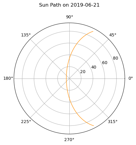
如果自己需要生成单个日期,这个是从之前的数据中取的。
# 修改时间范围为单日(示例使用2019-06-21)
single_day = '2019-06-21'
times = pd.date_range(f'{single_day} 00:00:00', f'{single_day} 23:59:00', freq='5min', tz=tz)# 移除夜间数据(保持原逻辑)
solpos = solarposition.get_solarposition(times, lat, lon)
solpos = solpos.loc[solpos['apparent_elevation'] > 0, :]ax = plt.subplot(1, 1, 1, projection='polar')
# 将散点图改为折线图
ax.plot(np.radians(solpos.azimuth), solpos.apparent_zenith,linewidth=1, color='darkorange',label=single_day)# ... 保留坐标轴设置代码 ...# 添加标题
plt.title(f'Sun Path on {single_day}', pad=20)
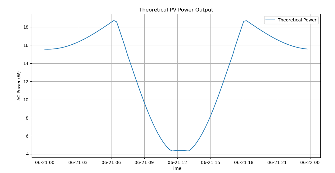
如何讨论针对某个地区日照情况
import numpy as np
import pandas as pd
import pvlib
from pvlib import solarposition, irradiance, atmosphere, pvsystem
from pvlib.location import Location
from pvlib.modelchain import ModelChain
import matplotlib.pyplot as plt# 1. 定义地理位置(纬度,经度,时区,海拔)
latitude = -36.11  # 纬度(°)
longitude = 146.84  # 经度(°)
# timezone = 'Asia/Shanghai'  # 时区
#
timezone = 'Australia/Sydney'
altitude = 159  # 海拔(m)# 创建Location对象
site = Location(latitude, longitude, timezone, altitude, name='Wodonga')# 2. 定义时间范围(这里以2023年某一天为例)
times = pd.date_range('2021-06-21 00:00', '2021-06-21 23:59', freq='15min', tz=timezone)# 3. 计算太阳位置
solpos = solarposition.get_solarposition(times, latitude, longitude)# 4. 计算大气层外辐照度(理论最大辐照度)
dni_extra = irradiance.get_extra_radiation(times)# 5. 计算理论辐照度(不考虑大气衰减)
# 使用大气层顶模型
# 计算总辐照度,需要先计算散射辐射和直接辐射
dhi = dni_extra * 0.1  # 假设散射辐射约为直接辐射的10%
ghi = dni_extra * np.cos(np.radians(solpos['apparent_zenith']))  # 计算全局水平辐照度irradiance_theoretical = irradiance.get_total_irradiance(surface_tilt=30,  # 倾斜角度(°)surface_azimuth=0,  # 方位角(180°为正南)solar_zenith=solpos['apparent_zenith'],solar_azimuth=solpos['azimuth'],dni=dni_extra,  # 使用大气层外直接辐射ghi=ghi,  # 添加全局水平辐照度dhi=dhi,  # 添加散射水平辐照度dni_extra=dni_extra,model='isotropic'
)
# 6. 定义光伏系统参数
sandia_modules = pvlib.pvsystem.retrieve_sam('SandiaMod')
sandia_module = sandia_modules['Canadian_Solar_CS5P_220M___2009_']
cec_inverters = pvlib.pvsystem.retrieve_sam('cecinverter')
cec_inverter = cec_inverters['ABB__MICRO_0_25_I_OUTD_US_208__208V_']# 7. 创建系统模型
system = pvlib.pvsystem.PVSystem(surface_tilt=30,surface_azimuth=180,module_parameters=sandia_module,inverter_parameters=cec_inverter,modules_per_string=1,strings_per_inverter=1,racking_model='open_rack',module_type='glass_polymer'
)# 8. 创建模型链
mc = ModelChain(system, site)# 9. 运行模型计算理论发电功率
weather = pd.DataFrame({'dni': irradiance_theoretical['poa_direct'],'ghi': irradiance_theoretical['poa_global'],'dhi': irradiance_theoretical['poa_diffuse'],'temp_air': 25,  # 假设恒温25°C'wind_speed': 1  # 假设风速1m/s
}, index=times)mc.run_model(weather)# 10. 获取理论发电功率
theoretical_power = mc.results.ac# 可视化结果
plt.figure(figsize=(12, 6))
plt.plot(theoretical_power.index, theoretical_power, label='Theoretical Power')
plt.xlabel('Time')
plt.ylabel('AC Power (W)')
plt.title('Theoretical PV Power Output')
plt.legend()
plt.grid()
plt.show()
使用这个计算功率,此处使用的是南半球。