多元回归的置信区间
本文是实验设计与分析(第6版,Montgomery著傅珏生译)第10章拟合回归模型第10.5节的python解决方案。本文尽量避免重复书中的理论,着于提供python解决方案,并与原书的运算结果进行对比。您可以从Detail 下载实验设计与分析(第6版,Montgomery著傅珏生译)电子版。本文假定您已具备python基础,如果您还没有python的基础,可以从Detail 下载相关资料进行学习。
我们常常要对回归系数{Bj}以及回归模型中其他感兴趣的量构造置信区间估计。这些置信区间的推导过程需要假定误差{εi}服从均值为零、方差为σ2的独立的正态分布,与10.4节的假设检验中的假定相同。
10.5.1单个回归系数的置信区间
因为最小二乘估计量![]() 是观测的线性组合,所以,
是观测的线性组合,所以,![]() 服从均值为
服从均值为![]() 、协方差矩阵为
、协方差矩阵为![]() 的正态分布。故统计量
的正态分布。故统计量
![]()
服从自由度为n-p的t分布,这里,![]() 是矩阵
是矩阵![]() 的第(jj)个元素,
的第(jj)个元素,![]() 是由(10.17)式得到的误差方差的估计。因此,回归系数
是由(10.17)式得到的误差方差的估计。因此,回归系数![]() 的100(1-α)%置信区间是
的100(1-α)%置信区间是
![]()
因为![]() ,这个置信区间也可写成
,这个置信区间也可写成
![]()
例10.7求例10.1中β1的95%置信区间。现在![]() ,由
,由![]() ,C11=1.429184×10⁻³,可得
,C11=1.429184×10⁻³,可得
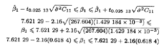
故β1的95%置信区间是
![]()
>>> print(model.summary2())
C:\Users\Administrator\AppData\Local\Programs\Python\Python311\Lib\site-packages\scipy\stats\_stats_py.py:1736: UserWarning: kurtosistest only valid for n>=20 ... continuing anyway, n=16
warnings.warn("kurtosistest only valid for n>=20 ... continuing "
Results: Ordinary least squares
====================================================================
Model: OLS Adj. R-squared: 0.916
Dependent Variable: df.Viscosity AIC: 137.5159
Date: 2024-03-14 10:31 BIC: 139.8337
No. Observations: 16 Log-Likelihood: -65.758
Df Model: 2 F-statistic: 82.50
Df Residuals: 13 Prob (F-statistic): 4.10e-08
R-squared: 0.927 Scale: 267.60
--------------------------------------------------------------------
Coef. Std.Err. t P>|t| [0.025 0.975]
--------------------------------------------------------------------
Intercept 1566.0778 61.5918 25.4267 0.0000 1433.0167 1699.1388
df.Temperature 7.6213 0.6184 12.3236 0.0000 6.2853 8.9573
df.Catalyst 8.5848 2.4387 3.5203 0.0038 3.3164 13.8533
--------------------------------------------------------------------
Omnibus: 1.215 Durbin-Watson: 2.607
Prob(Omnibus): 0.545 Jarque-Bera (JB): 0.779
Skew: -0.004 Prob(JB): 0.677
Kurtosis: 1.919 Condition No.: 1385
====================================================================
Notes:
[1] Standard Errors assume that the covariance matrix of the errors
is correctly specified.
[2] The condition number is large, 1.38e+03. This might indicate
that there are strong multicollinearity or other numerical
problems.
>>> print(model.params)
Intercept 1566.077771
df.Temperature 7.621290
df.Catalyst 8.584846
dtype: float64
>>> anovatable=sm.stats.anova_lm(model)
>>> anovatable
df sum_sq mean_sq F PR(>F)
df.Temperature 1.0 40840.842466 40840.842466 152.616757 1.473645e-08
df.Catalyst 1.0 3316.244074 3316.244074 12.392360 3.764806e-03
Residual 13.0 3478.850960 267.603920 NaN NaN
10.5.2平均响应的置信区间
我们还可以得到在特定点(比如x01,x02,…,x0k)上响应均值的置信区间。首先,设向量
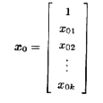
在该点的平均响应为
![]()
在该点的平均响应的估计为
![]()
因为![]() ,所以这个估计量是无偏的。
,所以这个估计量是无偏的。 ![]() 的方差为
的方差为
![]()
因此,在点x01,x02,…,x0k处的平均响应的100(1一a)%置信区间是
![]()