机器学习基础课程-6-课程实验
目录
6.1 实验介绍
实验准备
贷款审批结果预测
6.2 数据读取
6.3 数据处理
6.4 特征处理
有序型特征处理
类别型特征处理
数值型特征归一化
6.5 建立机器学习模型
建立测试模型
结果可视化
6.1 实验介绍
贷款审批结果预测
银行的放贷审批,核心要素为风险控制。因此,对于申请人的审查关注的要点为违约可能性。而违约可能性通常由申请人收入情况、稳定性、贷款数额及偿还年限等因素来衡量。该项目根据申请人条件,进一步细化得到各个变量对于违约评估的影响,从而预测银行是否会批准贷款申请。在项目实现过程中使用了经典的机器学习算法,对申请贷款客户进行科学归类,从而帮助金融机构提高对贷款信用风险的控制能力。
6.2 数据读取
数据读取
import pandas as pd
file = './data/loan_records.csv'
loan_df = pd.read_csv(file)
数据预览
print('数据集一共有{}行,{}列'.format(loan_df.shape[0], loan_df.shape[1]))
数据集一共有614行,13列
loan_df.head()
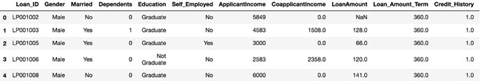
从贷款数据样本中,可以观察得到数据的特征
- Loan_ID:样本标号
- 性别:贷款人性别
- 已婚:是否结婚 (Y/N)
- 家属:供养人数
- 教育: 受教育程度(研究生/非研究生)
- Self_Employed:是否自雇 (Y/N)
- 申请人收入:申请人收入
- 共同申请人收入:联合申请人收入
- 贷款金额:贷款金额(单位:千)
- Loan_Amount_Term:贷款期限(单位:月)
- Credit_History:历史信用是否达标(0/1)
- Property_Area:居住地区(城市/半城市/农村)
- Loan_Status:是否批准(Y/N)
在我们即将构建的机器学习模型当中,Loan_Status将是模型训练的目标列
数据统计信息
loan_df.describe()
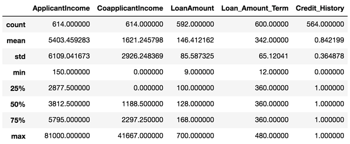
观察数据情况可以得知:
- LoanAmount、Loan_Amount_Term、Credit_History有明显的缺失值,需要进行空值处理
6.3 数据处理
重复值处理
if loan_df[loan_df['Loan_ID'].duplicated()].shape[0] > 0:
print('数据集存在重复样本')
else:
print('数据集不存在重复样本')
数据集不存在重复样本
缺失值处理
cols = loan_df.columns.tolist()
for col in cols:
empty_count = loan_df[col].isnull().sum()
print('{} 空记录数为:{}'.format(col, empty_count))
Loan_ID 空记录数为:0
Gender 空记录数为:13
Married 空记录数为:3
Dependents 空记录数为:15
Education 空记录数为:0
Self_Employed 空记录数为:32
ApplicantIncome 空记录数为:0
CoapplicantIncome 空记录数为:0
LoanAmount 空记录数为:22
Loan_Amount_Term 空记录数为:14
Credit_History 空记录数为:50
Property_Area 空记录数为:0
Loan_Status 空记录数为:0
# 将存在空值的样本删除
clean_loan_df = loan_df.dropna()
print('原始样本数为{},清理后的样本数为{}'.format(loan_df.shape[0], clean_loan_df.shape[0]))
原始样本数为614,清理后的样本数为480
特殊值处理
数值列Dependents包含3+,将其全部转换为3
# 可忽略SettingWithCopyWarning
clean_loan_df.loc[clean_loan_df['Dependents'] == '3+', 'Dependents'] = 3
特征数据和标签数据提取
在该数据集中,共有以下三种特征列
- 数值型特征列
-
- 家属:供养人数
- 申请人收入:申请人收入
- 共同申请人收入:联合申请人收入
- 贷款金额:贷款金额(单位:千)
- Loan_Amount_Term:贷款期限(单位:月)
- 有序型特征
-
- 教育: 受教育程度(研究生/非研究生)
- Credit_History:历史信用是否达标(0/1)
- 类别型特征
-
- 性别:贷款人性别
- 已婚:是否结婚 (Y/N)
- Self_Employed:是否自雇 (Y/N)
- Property_Area:居住地区(城市/半城市/农村)
# 按数据类型指定特征列
# 1. 数值型特征列
num_cols = ['Dependents', 'ApplicantIncome', 'CoapplicantIncome', 'LoanAmount', 'Loan_Amount_Term']
# 2. 有序型特征
ord_cols = ['Education', 'Credit_History']
# 3. 类别型特征
cat_cols = ['Gender', 'Married', 'Self_Employed', 'Property_Area']
feat_cols = num_cols + ord_cols + cat_cols
# 特征数据
feat_df = clean_loan_df[feat_cols]
#################################################################
# TODO
# 将标签Y转换为1,标签N转换为0
# 并将结果保存至labels变量中
labels = clean_loan_df['Loan_Status'].copy()
labels.loc[clean_loan_df['Loan_Status'] == 'Y'] = 1
labels.loc[clean_loan_df['Loan_Status'] == 'N'] = 0
#################################################################
现在我们需要划分数据集为训练集和测试集
from sklearn.model_selection import train_test_split
X_train, X_test, y_train, y_test = train_test_split(feat_df, labels, random_state=10, test_size=1/4)
print('训练集有{}条记录,测试集有{}条记录'.format(X_train.shape[0], X_test.shape[0]))
训练集有360条记录,测试集有120条记录
6.4 特征处理
有序型特征处理
有序型特征中Credit_History已经是数值,只需要转换教育列就即可:将Graduate转为1,Not Graduate转为0
# 可忽略SettingWithCopyWarning# 在训练集上做处理X_train.loc[X_train['Education'] == 'Graduate', 'Education'] = 1X_train.loc[X_train['Education'] == 'Not Graduate', 'Education'] = 0# 在测试集上做处理X_test.loc[X_test['Education'] == 'Graduate', 'Education'] = 1X_test.loc[X_test['Education'] == 'Not Graduate', 'Education'] = 0# 获取有序型特征处理结果train_ord_feats = X_train[ord_cols].valuestest_ord_feats = X_test[ord_cols].values类别型特征处理
from sklearn.preprocessing import LabelEncoder, OneHotEncoderimport numpy as npdef encode_cat_feats(train_df, test_df, col_name): """ 对某列类别型数据进行编码 """ # 类别型数据 train_cat_feat = X_train[col_name].values test_cat_feat = X_test[col_name].values label_enc = LabelEncoder() onehot_enc = OneHotEncoder(sparse=False) # 在训练集上处理 proc_train_cat_feat = label_enc.fit_transform(train_cat_feat).reshape(-1, 1) proc_train_cat_feat = onehot_enc.fit_transform(proc_train_cat_feat) # 在测试集上处理 proc_test_cat_feat = label_enc.transform(test_cat_feat).reshape(-1, 1) proc_test_cat_feat = onehot_enc.transform(proc_test_cat_feat) return proc_train_cat_feat, proc_test_cat_feat# 初始化编码处理后的特征enc_train_cat_feats = Noneenc_test_cat_feats = None# 对每个类别型特征进行编码处理for cat_col in cat_cols: enc_train_cat_feat, enc_test_cat_feat = encode_cat_feats(X_train, X_test, cat_col) # 在训练数据上合并特征 if enc_train_cat_feats is None: enc_train_cat_feats = enc_train_cat_feat else: enc_train_cat_feats = np.hstack((enc_train_cat_feats, enc_train_cat_feat)) # 在测试数据上合并特征 if enc_test_cat_feats is None: enc_test_cat_feats = enc_test_cat_feat else: enc_test_cat_feats = np.hstack((enc_test_cat_feats, enc_test_cat_feat))数值型特征归一化
将所有特征进行合并,然后进行范围归一化。
from sklearn.preprocessing import MinMaxScaler# 获取数值型特征train_num_feats = X_train[num_cols].valuestest_num_feats = X_test[num_cols].values# 合并序列型特征、类别型特征、数值型特征all_train_feats = np.hstack((train_ord_feats, enc_train_cat_feats, train_num_feats))all_test_feats = np.hstack((test_ord_feats, enc_test_cat_feats, test_num_feats))################################################################## TODO# 数值归一化到0-1# 将处理后的训练特征保存到变量all_proc_train_feats中# 将处理后的测试特征保存到变量all_proc_test_feats中scaler = MinMaxScaler(feature_range=(0, 1))all_proc_train_feats = scaler.fit_transform(all_train_feats)all_proc_test_feats = scaler.transform(all_test_feats)#################################################################print('处理后的特征维度为', all_proc_train_feats.shape[1])处理后的特征维度为 166.5 建立机器学习模型
建立测试模型
使用网格搜索(GridSearchCV)来调整模型的重要参数
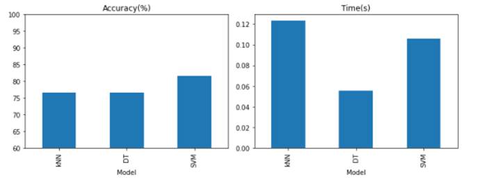
from sklearn.linear_model import LogisticRegressionfrom sklearn.neighbors import KNeighborsClassifierfrom sklearn.tree import DecisionTreeClassifierfrom sklearn.svm import SVCfrom sklearn.model_selection import GridSearchCVimport timedef train_test_model(X_train, y_train, X_test, y_test, model_name, model, param_range): """ 训练并测试模型 model_name: kNN kNN模型,对应参数为 n_neighbors LR 逻辑回归模型,对应参数为 C SVM 支持向量机,对应参数为 C DT 决策树,对应参数为 max_depth Stacking 将kNN, SVM, DT集成的Stacking模型, meta分类器为LR AdaBoost AdaBoost模型,对应参数为 n_estimators GBDT GBDT模型,对应参数为 learning_rate RF 随机森林模型,对应参数为 n_estimators 根据给定的参数训练模型,并返回 1. 最优模型 2. 平均训练耗时 3. 准确率 """ print('训练{}...'.format(model_name)) ################################################################# # TODO # 初始化网格搜索方法进行模型训练,使用5折交叉验证,保存到变量clf中 clf = GridSearchCV(estimator=model, param_grid=param_range, cv=5, scoring='accuracy', refit=True) start = time.time() clf.fit(X_train, y_train) ################################################################# start = time.time() clf.fit(X_train, y_train) # 计时 end = time.time() duration = end - start print('耗时{:.4f}s'.format(duration)) # 验证模型 train_score = clf.score(X_train, y_train) print('训练准确率:{:.3f}%'.format(train_score * 100)) test_score = clf.score(X_test, y_test) print('测试准确率:{:.3f}%'.format(test_score * 100)) print('训练模型耗时: {:.4f}s'.format(duration)) y_pred = clf.predict(X_test) return clf, test_score, duration################################################################## TODO# 在model_name_param_dict中添加逻辑回归和SVM分类器,并指定相应的超参数及搜索范围model_name_param_dict = {'kNN': (KNeighborsClassifier(), {'n_neighbors': [1, 5, 15]}), 'DT': (DecisionTreeClassifier(), {'max_depth': [10, 50, 100]}), 'SVM': (SVC(kernel='linear'), {'C': [0.01, 1, 100]}), 'DT': (DecisionTreeClassifier(), {'max_depth': [10, 50, 100]}) }################################################################## 比较结果的DataFrameresults_df = pd.DataFrame(columns=['Accuracy (%)', 'Time (s)'], index=list(model_name_param_dict.keys()))results_df.index.name = 'Model'for model_name, (model, param_range) in model_name_param_dict.items(): _, best_acc, mean_duration = train_test_model(all_proc_train_feats, y_train.astype('int'), all_proc_test_feats, y_test.astype('int'), model_name, model, param_range) results_df.loc[model_name, 'Accuracy (%)'] = best_acc * 100 results_df.loc[model_name, 'Time (s)'] = mean_duration训练kNN...耗时0.0661s训练准确率:80.556%测试准确率:76.667%训练模型耗时: 0.0661s训练DT...耗时0.0442s训练准确率:91.111%测试准确率:76.667%训练模型耗时: 0.0442s训练SVM...耗时0.1124s训练准确率:80.556%测试准确率:81.667%训练模型耗时: 0.1124s结果可视化
现在对比一下各个模型的效率和他们的准确率吧!
# 结果可视化import matplotlib.pyplot as plt%matplotlib inlineplt.figure(figsize=(10, 4))ax1 = plt.subplot(1, 2, 1)results_df.plot(y=['Accuracy (%)'], kind='bar', ylim=[60, 100], ax=ax1, title='Accuracy(%)', legend=False)ax2 = plt.subplot(1, 2, 2)results_df.plot(y=['Time (s)'], kind='bar', ax=ax2, title='Time(s)', legend=False)plt.tight_layout()plt.show()