当前位置：首页 > news >正文

第 2.3 节: 基于 Python 的关节空间与任务空间控制

news 来源：原创 2025/5/2 8:08:44

在机器人控制领域，我们通常关心两个主要的“空间”：关节空间（Joint Space）和任务空间（Task Space，也常称为操作空间 Operational Space）。关节空间描述了机器人各关节的角度或位置集合，是机器人硬件直接控制的量。而任务空间描述了机器人末端执行器（End-effector）在三维空间中的位置和姿态，这通常是我们希望机器人完成任务时的目标。

本节我们将回顾机器人正逆运动学的基础，探讨如何使用 Python 实现这些计算，并介绍基于 PID 控制器的关节控制和基本的任务空间控制概念及实践。

2.3.1 机器人正逆运动学回顾与 Python 实现

什么是正运动学 (Forward Kinematics - FK)?

正运动学解决的问题是：给定机器人所有关节的角度（或位置），计算出机器人末端执行器在基本坐标系中的位置和姿态。 简单来说，就是“我知道关节怎么动，我想知道爪子（或脚）在哪里”。

正运动学通常通过一系列齐次变换矩阵（Homogeneous Transformation Matrices）来描述，这些矩阵根据每个关节的运动和连杆的几何形状构建。连接基坐标系到末端执行器的所有变换矩阵的乘积就是末端执行器相对于基坐标系的位姿矩阵。

什么是逆运动学 (Inverse Kinematics - IK)?

逆运动学解决的问题是：给定机器人末端执行器在基本坐标系中期望的位置和姿态，计算出机器人所有关节需要设置的角度（或位置）。 简单来说，就是“我知道爪子（或脚）应该在哪里，我想知道每个关节应该怎么转”。

与正运动学不同，逆运动学通常更复杂，可能存在多个解、无解或奇异构型（Singularity）问题。常用的解决方法包括：

解析解 (Analytical Solutions): 对于结构简单的机器人（如许多串联机械臂），可以通过几何或代数方法直接推导出关节角度的公式。这是最快、最准确的方法，但只适用于特定构型。
数值解 (Numerical Solutions): 对于更复杂的机器人，通常使用迭代优化方法来寻找逆运动学解。这些方法通过不断调整关节角度，最小化当前末端执行器位姿与目标位姿之间的误差，直到误差足够小。常见的数值方法有牛顿法、梯度下降法等。

Python 实现：PyKDL vs SciPy

PyKDL (Python Bindings for Orocos KDL): Orocos Kinematics and Dynamics Library (KDL) 是一个 C++ 库，PyKDL 提供了其 Python 接口。KDL 专门为机器人学设计，提供了丰富的功能，包括 FK, IK, Jacobian, Dynamics 等。如果你的机器人模型复杂且需要进行动力学计算，或者追求更高的性能，PyKDL 是一个很好的选择。安装可能稍微复杂一些。
SciPy: SciPy 是一个强大的 Python 科学计算库，其中的 scipy.spatial.transform 模块可以方便地进行三维空间中的旋转和平移变换，scipy.optimize 模块提供了各种优化算法，非常适合用于求解数值逆运动学问题。SciPy 通常更容易安装和使用，对于理解数值 IK 的原理很有帮助。

在本节的实践中，考虑到易用性和通用性，我们将使用 SciPy 来实现简化的 G1 单腿的 FK 和数值 IK。

2.3.1.1 G1 单腿简化模型与运动学计算

我们以 Unitree G1 的一条腿为例进行简化。假设腿部有三个主要关节用于实现空间中的位置控制：髋关节俯仰 (Hip Pitch)、大腿关节俯仰 (Thigh Pitch) 和小腿关节俯仰 (Calf Pitch)。我们忽略髋关节的横滚/偏航以及脚踝关节，将模型简化为在侧向平面内运动的 3-DOF 机械腿。

模型参数 (示例):

髋关节到大腿关节的垂直偏移 (y 方向): hip_offset_y
大腿长度: thigh_length
小腿长度: calf_length

Python

import numpy as np
from scipy.spatial.transform import Rotation as R
from scipy.optimize import minimize# 假设的 G1 单腿简化模型参数 (单位: 米)
# 注意：这些值是示例，可能与实际 G1 机器人参数不同
HIP_OFFSET_Y = 0.1  # 髋关节到大腿关节的垂直偏移
THIGH_LENGTH = 0.3  # 大腿长度
CALF_LENGTH = 0.3   # 小腿长度# 关节顺序：[Hip Pitch, Thigh Pitch, Calf Pitch] (弧度)
# 基本坐标系位于髋关节处def fk_leg(joint_angles):"""简化单腿的正运动学计算。假设关节顺序为 [hip_pitch, thigh_pitch, calf_pitch]。所有关节旋转轴平行于Y轴 (侧向)，旋转绕自身关节原点进行。"""hip_pitch, thigh_pitch, calf_pitch = joint_angles# 1. 从基本坐标系到髋关节俯仰轴末端 (考虑髋关节偏移)# 这里简化处理，假设髋关节偏移只影响初始平移T0_hip = np.eye(4)T0_hip[1, 3] = -HIP_OFFSET_Y # 假设髋关节中心在基座下方 Y 轴负方向偏移# 2. 髋关节俯仰旋转 (绕Y轴)R_hip = R.from_euler('y', hip_pitch).as_matrix()T_hip_joint = np.eye(4)T_hip_joint[:3, :3] = R_hip# 关节旋转通常不带平移，平移是连杆的长度# 3. 髋关节俯仰轴末端到大腿关节 (大腿的根部)# 忽略了髋关节的其他自由度，直接连接到大腿# 我们将髋关节的起始点作为连杆1的开始，大腿根部作为连杆1的结束# simplified: let's assume hip pitch rotates the base of the thigh link# T0_thigh_base = T0_hip @ T_hip_joint # This isn't quite right for standard DH# Let's redefine: Base is origin. Hip pitch joint is at origin.# Link 1 is a point at (0, -HIP_OFFSET_Y, 0) after the hip pitch rotation?# This is getting complex. Let's use a simpler DH-like thinking for this example.# Assume Hip Pitch is joint 1 at origin (0,0,0), rotating link 1.# Link 1 ends at (0, -HIP_OFFSET_Y, 0) *after* rotation. Then thigh starts there.# Simpler approach: Base frame -> Joint 1 (Hip Pitch) -> Link 1 (Thigh) -> Joint 2 (Thigh Pitch) -> Link 2 (Calf) -> Joint 3 (Calf Pitch) -> Link 3 (Foot).# Let's refine the FK chain:# Frame 0 (Base)# Frame 1 (after Hip Pitch, at origin, rotating around Y)# Frame 2 (after translating along Link 1 - conceptual short link to thigh joint)# Frame 3 (after Thigh Pitch, at thigh joint)# Frame 4 (after translating along Link 2 - thigh length)# Frame 5 (after Calf Pitch, at calf joint)# Frame 6 (after translating along Link 3 - calf length, end-effector)# Simpler simplified chain for this example:# Start at a point (0, -HIP_OFFSET_Y, 0) relative to base. This is the effective base of the 2-link leg.# Joint 1 (relative Hip Pitch) rotates Link 1 (Thigh).# Joint 2 (relative Thigh Pitch) rotates Link 2 (Calf) relative to Link 1.# Joint 3 (relative Calf Pitch) rotates End-effector relative to Link 2.# The angles hip_pitch, thigh_pitch, calf_pitch are relative angles.# Let's use a common convention: angles are relative to the *previous* link's frame,# and link lengths are along the Z axis of the *current* frame before rotation,# or translation along X after rotation... DH parameters are the standard way.# Without strict DH, let's just use sequential transformations assuming rotations are around Y.T0_1 = np.eye(4) # Transformation from Frame 0 to Frame 1 (at Hip Pitch joint) - assume originR1 = R.from_euler('y', hip_pitch).as_matrix()T1_2 = np.eye(4)T1_2[1, 3] = -HIP_OFFSET_Y # Translation from Hip Pitch joint to Thigh Pitch joint base (conceptually)T0_2 = T0_1 @ T1_2 # This places the effective leg base after hip offset# Now consider the 2-link arm part starting from T0_2 origin# Joint 2 is Thigh Pitch, rotates around Y# Link 2 is Thigh Length# Joint 3 is Calf Pitch, rotates around Y# Link 3 is Calf LengthT2_3 = np.eye(4) # Transformation from Frame 2 to Frame 3 (at Thigh Pitch joint) - origin of the 2-link leg partR3 = R.from_euler('y', thigh_pitch).as_matrix()T3_4 = np.eye(4)T3_4[2, 3] = THIGH_LENGTH # Translate along the Z-axis of Frame 3 by thigh length (assuming Z is forward/downwards)T0_4 = T0_2 @ T2_3 @ T3_4 # Position after Thigh link# Now add the Calf part# Joint 3 is Calf Pitch, rotates around Y# Link 3 is Calf LengthT4_5 = np.eye(4) # Transformation from Frame 4 to Frame 5 (at Calf Pitch joint) - origin of the calf linkR5 = R.from_euler('y', calf_pitch).as_matrix()T5_6 = np.eye(4)T5_6[2, 3] = CALF_LENGTH # Translate along the Z-axis of Frame 5 by calf lengthT0_6 = T0_4 @ T4_5 @ T5_6 # Final end-effector position# The position is the last column of the transformation matrixend_effector_pos = T0_6[:3, 3]return end_effector_pos# Example usage of FK
test_angles = np.array([np.deg2rad(0), np.deg2rad(0), np.deg2rad(0)]) # Stretched leg
pos = fk_leg(test_angles)
print(f"FK for angles {np.rad2deg(test_angles)} deg: Position = {pos}")test_angles = np.array([np.deg2rad(30), np.deg2rad(-45), np.deg2rad(90)])
pos = fk_leg(test_angles)
print(f"FK for angles {np.rad2deg(test_angles)} deg: Position = {pos}")

注意： 上述 fk_leg 实现是基于一个简化的、假设的连杆连接方式和平移/旋转顺序。实际机器人的 DH 参数或URDF模型会提供精确的变换。这里主要是为了演示如何在 Python 中进行基于变换矩阵的 FK 计算。旋转是使用 scipy.spatial.transform.Rotation 完成的，平移直接修改齐次变换矩阵的第四列。

2.3.1.2 数值逆运动学实现

数值逆运动学通过优化方法找到使 FK 输出接近目标位置的关节角度。我们定义一个目标函数，该函数计算当前关节角度下末端执行器位置与目标位置之间的欧几里得距离的平方，然后使用优化器最小化这个函数。

Python

# Objective function for IK
def objective_ik(joint_angles, target_pos):"""IK 优化问题的目标函数：计算当前关节角度下的末端执行器位置与目标位置之间的距离平方。"""current_pos = fk_leg(joint_angles)return np.sum((current_pos - target_pos)**2)def ik_leg(target_pos, initial_guess_angles, joint_limits=None):"""使用 SciPy 优化器求解单腿的逆运动学。"""# bounds (optional): list of tuples (min_angle, max_angle) for each joint# example bounds for G1 leg (approximate, in radians):# Hip Pitch: -1.57 to 1.57 (-90 to 90 deg)# Thigh Pitch: -2.61 to 0.61 (-150 to 35 deg)# Calf Pitch: -2.53 to -0.61 (-145 to -35 deg) # Note: Angles often relative# Let's provide example bounds, convert degrees to radians# Assuming the angles are relative pitches as in the FKexample_bounds_deg = [(-90, 90),  # Hip Pitch(-150, 35), # Thigh Pitch(-145, -35) # Calf Pitch (these might be relative angles or range)]example_bounds_rad = [(np.deg2rad(lower), np.deg2rad(upper)) for lower, upper in example_bounds_deg]# Use minimize from scipy.optimizeresult = minimize(objective_ik,initial_guess_angles, # 初始猜测值args=(target_pos,),    # 传递给目标函数的额外参数method='SLSQP',        # 选择一个优化方法，SLSQP是一个常用的选择bounds=joint_limits if joint_limits else example_bounds_rad, # 关节限制tol=1e-6               # 容忍度)if result.success:return result.x # 返回找到的关节角度else:print(f"Warning: IK failed to converge. Message: {result.message}")return None # 或返回初始猜测值，取决于需求# Example usage of IK
target_pos = np.array([0.0, -HIP_OFFSET_Y - 0.1, -0.5]) # Example target position
initial_angles = np.array([0, 0, 0]) # Start from stretched legik_solution = ik_leg(target_pos, initial_angles)if ik_solution is not None:print(f"\nTarget Position: {target_pos}")print(f"IK Solution (radians): {ik_solution}")print(f"IK Solution (degrees): {np.rad2deg(ik_solution)}")# Verify the FK of the IK solutionreached_pos = fk_leg(ik_solution)print(f"Reached Position with IK solution: {reached_pos}")print(f"Error distance: {np.linalg.norm(reached_pos - target_pos)}")
else:print("\nIK solution not found.")# Another IK example
target_pos_2 = np.array([0.0, -HIP_OFFSET_Y, -0.4]) # Different target
initial_angles_2 = np.deg2rad([10, -30, -60]) # Different initial guessik_solution_2 = ik_leg(target_pos_2, initial_angles_2)if ik_solution_2 is not None:print(f"\nTarget Position: {target_pos_2}")print(f"IK Solution 2 (radians): {ik_solution_2}")print(f"IK Solution 2 (degrees): {np.rad2deg(ik_solution_2)}")reached_pos_2 = fk_leg(ik_solution_2)print(f"Reached Position with IK solution 2: {reached_pos_2}")print(f"Error distance 2: {np.linalg.norm(reached_pos_2 - target_pos_2)}")
else:print("\nIK solution 2 not found.")

通过运行上述代码，我们可以看到如何使用 SciPy 的优化器求解给定目标位置的关节角度。需要注意的是，数值 IK 对初始猜测值敏感，且不能保证找到全局最优解或所有可能的解。关节限制 (bounds) 对于找到符合物理约束的解至关重要。

2.3.2 基于 PID 控制器实现关节位置/速度/力矩控制

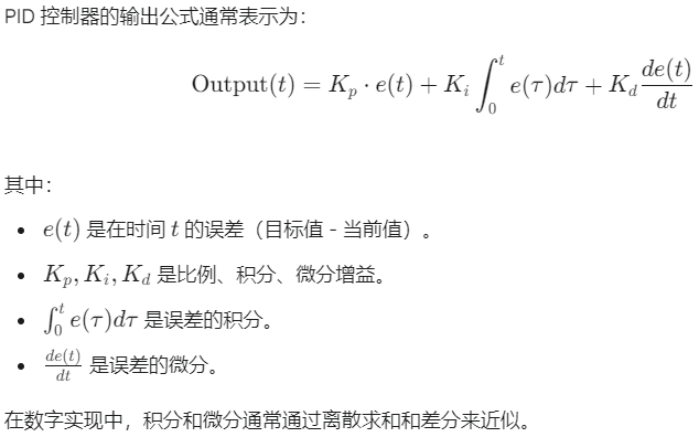
PID 控制器是一种经典且广泛应用于工业控制领域的反馈控制器。它根据系统误差（目标值与当前值之差）的比例 (P)、积分 (I) 和微分 (D) 来计算控制输出。

对于大多数具备关节力矩控制接口的机器人（如 Unitree G1），典型的控制架构是：位置环 (PID) -> 速度环 (PID) -> 力矩指令。外部位置指令通过位置环 PID 产生速度指令，速度指令通过速度环 PID 产生力矩指令，最终由电机的电流控制器产生力矩。但我们也可以直接使用一个 PID 控制器来输出力矩指令以达到目标位置或速度，这取决于系统的简化程度。

2.3.2.1 Python 实现一个通用的 PID 控制器类

我们可以创建一个 Python 类来实现一个可复用的 PID 控制器。

总结

本节我们回顾了机器人正逆运动学，并使用 SciPy 实现了简化的 G1 单腿 FK 和数值 IK。接着，我们实现了一个通用的 PID 控制器类，并在一个简化的关节位置控制仿真中进行了演示。最后，我们将 FK、IK 和 PID 控制器结合起来，展示了如何实现一个基于 IK 的基本任务空间位置控制。

在本节的实践中，我们将演示基于 IK 的基本任务空间位置控制，这是一种相对简单的实现方式，非常适合入门理解任务空间控制的概念。

2.4 Python 实践：G1 单腿的简单任务空间控制

我们将结合之前实现的 FK、IK 和 PID 控制器，编写一个脚本来控制简化的 G1 单腿模型达到一个指定的末端位置。

比例项 (P): 与当前误差成正比。误差越大，控制输出越大。提供即时响应。
积分项 (I): 与误差的累积（积分）成正比。用于消除稳态误差，即使误差很小，长时间累积的积分项也能产生足够的控制作用。
微分项 (D): 与误差的变化率（微分）成正比。用于预测误差的变化趋势，提供阻尼作用，减少超调和震荡
应用于机器人关节控制：
关节位置控制: 误差是目标关节角度与当前关节角度之差。PID 输出可以是关节力矩（电流）或关节速度指令，取决于机器人底层控制接口。
关节速度控制: 误差是目标关节速度与当前关节速度之差。PID 输出通常是关节力矩（电流）。
关节力矩控制: 误差是目标关节力矩与当前实际关节力矩之差（如果能测量）。这层控制通常在更底层，更常见的是将 PID 输出作为力矩指令。

Python

import timeclass PIDController:"""一个简单的 PID 控制器类。"""def __init__(self, Kp, Ki, Kd, setpoint):self.Kp = Kpself.Ki = Kiself.Kd = Kdself.setpoint = setpoint  # 目标值self.integral = 0self.previous_error = 0self.last_time = time.time() # 用于计算dtdef update(self, current_value):"""更新 PID 控制器并计算控制输出。current_value: 当前的系统值。"""current_time = time.time()dt = current_time - self.last_timeif dt <= 0: # 避免除以零或负dtreturn 0error = self.setpoint - current_value# Proportional termp_term = self.Kp * error# Integral termself.integral += error * dt# Optional: Integral windup prevention (clamping the integral term)# self.integral = max(min(self.integral, integral_max), integral_min) # Need to define integral_max/min# Derivative termderivative = (error - self.previous_error) / dtd_term = self.Kd * derivative# Update previous error and timeself.previous_error = errorself.last_time = current_time# Total outputoutput = p_term + self.integral * self.Ki + d_term# Optional: Output clamping# output = max(min(output, output_max), output_min) # Need to define output_max/minreturn outputdef set_setpoint(self, setpoint):"""设置新的目标值，并重置积分项以避免旧误差累积的影响。"""self.setpoint = setpointself.integral = 0 # Reset integral on setpoint changeself.previous_error = self.setpoint - self.setpoint # Reset previous error (should be 0)self.last_time = time.time() # Reset time for dt calculationdef reset(self):"""重置控制器状态。"""self.integral = 0self.previous_error = 0self.last_time = time.time()# Example usage of PID Controller (simulating a simple joint)
if __name__ == "__main__":# Simulate a single joint trying to reach a target angletarget_angle = np.deg2rad(45) # Target angle in radiansinitial_angle = np.deg2rad(0) # Starting angle# PID gains (need tuning based on the system dynamics)# These are example gains, likely need adjustment for a real robot jointkp = 2.0ki = 0.1kd = 0.5pid = PIDController(kp, ki, kd, target_angle)# Simple simulation parameterssimulation_time = 5.0 # secondsdt = 0.01 # simulation step timecurrent_angle = initial_anglecurrent_velocity = 0.0 # Simple simulation doesn't have complex dynamicsprint(f"Starting simulation for joint position control...")print(f"Target angle: {np.rad2deg(target_angle):.2f} deg")# In a real robot, you would read sensor data (current_angle, current_velocity)# Here, we simulate the effect of the control output on the angle.# A very simple model: control output is like a velocity command.# In a real system, output would be torque/voltage, affecting acceleration.time_steps = int(simulation_time / dt)for i in range(time_steps):# Get control output from PIDcontrol_output = pid.update(current_angle)# --- Simulate joint dynamics (very simple approximation) ---# Assume control_output acts like a velocity command for simplicity# A more realistic simulation would use F=ma, integrate acceleration to velocity, etc.current_angle += control_output * dt# In a real system, you'd send `control_output` (e.g., as torque) to the robot API# and read the new `current_angle` from sensors in the next loop iteration.# ---------------------------------------------------------# Print or log current stateif i % 50 == 0: # Print less frequentlyprint(f"Time: {i*dt:.2f}s, Current Angle: {np.rad2deg(current_angle):.2f} deg, Error: {np.rad2deg(pid.setpoint - current_angle):.2f} deg, Control Output: {control_output:.2f}")print(f"Simulation finished. Final angle: {np.rad2deg(current_angle):.2f} deg")

上述代码提供了一个简单的 PID 控制器类及其在一个简化仿真环境中的使用示例。请注意，模拟关节动力学部分是高度简化的，仅用于演示 PID 控制器的基本工作方式。在实际机器人控制中，你需要与机器人 SDK 或控制接口交互，发送控制指令（如力矩、速度或位置指令，取决于接口），并读取真实的关节传感器数据。PID 增益 Kp,Ki,Kd 的选取（PID 调参）对于实现稳定和快速的控制至关重要，通常需要通过实验或更高级的方法来确定。

2.3.3 基本任务空间控制概念

任务空间控制的目标是直接控制机器人的末端执行器在笛卡尔空间（3D 位置和姿态）中的运动。与关节空间控制直接操作关节角度不同，任务空间控制需要一个额外的层来处理关节空间和任务空间之间的转换，通常依赖于正逆运动学和雅可比矩阵。

实现基本任务空间控制的常见方法：

基于逆运动学 (IK-based) 的方法:
- 原理: 给定一个目标任务空间位姿，使用逆运动学计算达到该位姿所需的关节角度。
- 控制: 然后使用关节空间控制器（如上面实现的 PID）来驱动机器人关节到达这些计算出的关节角度。
- 优点: 概念简单，易于实现。
- 缺点:
  - 逆运动学可能没有解析解，需要数值求解，计算量可能较大。
  - 逆运动学解可能不唯一，需要选择合适的解。
  - 在运动过程中，如果频繁计算 IK，可能会导致运动不平滑，特别是在接近奇异点时。
  - 这种方法本质上是在控制关节位置，任务空间的轨迹跟踪性能受 IK 求解频率和关节控制器性能限制。
基于雅可比 (Jacobian-based) 的方法:
- 原理: 利用机器人雅可比矩阵（Jacobian Matrix）来建立关节速度和任务空间速度之间的关系 (x˙=J(q)q˙，其中 x˙ 是任务空间速度，q˙ 是关节速度，J(q) 是雅可比矩阵，依赖于关节角度 q）。
- 控制: 通过计算期望的任务空间速度，并利用雅可比矩阵（或其伪逆）求解所需的关节速度，然后控制关节速度。也可以结合任务空间的误差直接计算所需的关节速度，例如使用任务空间 PID 控制器。
- 优点: 可以实现更平滑的运动，更适合轨迹跟踪，能够更好地处理奇异点（通过各种雅可比伪逆方法）。
- 缺点: 需要计算和更新雅可比矩阵，处理奇异点需要更复杂的算法。
简化模型和动力学: 这里的腿部模型和关节动力学是高度简化的。实际机器人具有复杂的动力学特性，需要更精确的模型和更鲁棒的控制器。
IK 计算频率: 在每个时间步都计算 IK 可能计算量较大，且 IK 的解质量会影响控制效果。更高级的任务空间控制（如基于雅可比的方法）通常更高效。
无姿态控制: 这个例子只控制了末端执行器的位置，没有控制其姿态。在任务空间控制中，通常需要控制末端执行器的 6-DOF 位姿 (x, y, z, roll, pitch, yaw)。IK 和 Jacobian 方法都可以扩展到 6-DOF。
无碰撞检测和避障: 实际机器人控制需要考虑环境中障碍物，避免碰撞。
单腿 vs 双腿/全身: G1 是一个双足机器人，控制全身运动（包括平衡、步态生成）远比控制单腿复杂，需要考虑多个腿的协调、质心控制等。

Python

import numpy as np
import time
from scipy.spatial.transform import Rotation as R
from scipy.optimize import minimize # Already imported# Assuming the FK, IK, and PIDController definitions from previous sections are available
# (Copy and paste the code for HIP_OFFSET_Y, THIGH_LENGTH, CALF_LENGTH, fk_leg, objective_ik, ik_leg, PIDController here)# --- Copy FK, IK, and PIDController definitions from above ---
HIP_OFFSET_Y = 0.1
THIGH_LENGTH = 0.3
CALF_LENGTH = 0.3def fk_leg(joint_angles):hip_pitch, thigh_pitch, calf_pitch = joint_anglesT0_1 = np.eye(4)R1 = R.from_euler('y', hip_pitch).as_matrix()T1_2 = np.eye(4)T1_2[1, 3] = -HIP_OFFSET_YT0_2 = T0_1 @ T1_2T2_3 = np.eye(4)R3 = R.from_euler('y', thigh_pitch).as_matrix()T3_4 = np.eye(4)T3_4[2, 3] = THIGH_LENGTHT0_4 = T0_2 @ T2_3 @ T3_4T4_5 = np.eye(4)R5 = R.from_euler('y', calf_pitch).as_matrix()T5_6 = np.eye(4)T5_6[2, 3] = CALF_LENGTHT0_6 = T0_4 @ T4_5 @ T5_6return T0_6[:3, 3]def objective_ik(joint_angles, target_pos):current_pos = fk_leg(joint_angles)return np.sum((current_pos - target_pos)**2)def ik_leg(target_pos, initial_guess_angles, joint_limits=None):example_bounds_deg = [(-90, 90), (-150, 35), (-145, -35)]example_bounds_rad = [(np.deg2rad(lower), np.deg2rad(upper)) for lower, upper in example_bounds_deg]result = minimize(objective_ik,initial_guess_angles,args=(target_pos,),method='SLSQP',bounds=joint_limits if joint_limits else example_bounds_rad,tol=1e-6)if result.success:return result.xelse:# print(f"Warning: IK failed to converge. Message: {result.message}")return initial_guess_angles # Return last valid angles or initial guessclass PIDController:def __init__(self, Kp, Ki, Kd, setpoint):self.Kp = Kpself.Ki = Kiself.Kd = Kdself.setpoint = setpointself.integral = 0self.previous_error = 0self.last_time = time.time()def update(self, current_value):current_time = time.time()dt = current_time - self.last_timeif dt <= 0:dt = 1e-6 # Prevent division by zeroerror = self.setpoint - current_valuep_term = self.Kp * errorself.integral += error * dtderivative = (error - self.previous_error) / dtd_term = self.Kd * derivativeself.previous_error = errorself.last_time = current_timeoutput = p_term + self.integral * self.Ki + d_termreturn outputdef set_setpoint(self, setpoint):self.setpoint = setpointself.integral = 0self.previous_error = self.setpoint - self.setpointself.last_time = time.time()def reset(self):self.integral = 0self.previous_error = 0self.last_time = time.time()
# --- End of copy-pasted definitions ---# Task Space Control Simulation Parameters
target_task_pos = np.array([0.0, -HIP_OFFSET_Y - 0.1, -0.5]) # Target end-effector position
# target_task_pos = np.array([0.0, -HIP_OFFSET_Y - 0.2, -0.4]) # Another targetsimulation_time = 10.0 # seconds
dt = 0.01 # simulation step time# Initial state
current_joint_angles = np.deg2rad([0, 0, 0]) # Start from stretched leg
current_task_pos = fk_leg(current_joint_angles)# PID controllers for each joint (tuned for joint position control)
# These gains will likely need tuning for your specific simulation/robot model
# Example gains (arbitrary, need real tuning)
joint_kp = 5.0
joint_ki = 0.2
joint_kd = 1.0pid_hip_pitch = PIDController(joint_kp, joint_ki, joint_kd, current_joint_angles[0])
pid_thigh_pitch = PIDController(joint_kp, joint_ki, joint_kd, current_joint_angles[1])
pid_calf_pitch = PIDController(joint_kp, joint_ki, joint_kd, current_joint_angles[2])print(f"Starting task space control simulation...")
print(f"Initial Joint Angles (deg): {np.rad2deg(current_joint_angles)}")
print(f"Initial Task Position: {current_task_pos}")
print(f"Target Task Position: {target_task_pos}")time_steps = int(simulation_time / dt)# Simple simulation loop
# In each step, we:
# 1. Calculate the required joint angles using IK for the target task position.
# 2. Set these angles as the setpoints for the joint PID controllers.
# 3. Update the joint angles based on the PID outputs (simplified dynamics).
# 4. Recalculate the current task position using FK.for i in range(time_steps):# --- Task Space Control Logic ---# Calculate target joint angles using IK for the desired task position# We use the current_joint_angles as the initial guess for IKdesired_joint_angles = ik_leg(target_task_pos, current_joint_angles)if desired_joint_angles is None:print(f"Time {i*dt:.2f}s: IK failed. Skipping control update.")# In a real system, you might have strategies to handle IK failurecontinue # Skip this step if IK fails# Set the new target angles for the joint PID controllerspid_hip_pitch.set_setpoint(desired_joint_angles[0])pid_thigh_pitch.set_setpoint(desired_joint_angles[1])pid_calf_pitch.set_setpoint(desired_joint_angles[2])# --- End Task Space Control Logic ---# --- Simulate Joint Control (using PID) and Robot Dynamics ---# Get control outputs for each joint PIDcontrol_hip = pid_hip_pitch.update(current_joint_angles[0])control_thigh = pid_thigh_pitch.update(current_joint_angles[1])control_calf = pid_calf_pitch.update(current_joint_angles[2])# Apply control outputs to simulate joint movement# Again, this is a very simple model. Control output is like a velocity command.# A real system would integrate torques to get acceleration, then velocity, then position.current_joint_angles[0] += control_hip * dtcurrent_joint_angles[1] += control_thigh * dtcurrent_joint_angles[2] += control_calf * dt# In a real system, you would send control_outputs (e.g., as torques/voltages)# to the robot's motor controllers via its API and read new joint angles.# ---------------------------------------------------------------# Update current task position based on new joint anglescurrent_task_pos = fk_leg(current_joint_angles)# Print or log current stateif i % 100 == 0: # Print less frequentlytask_error = np.linalg.norm(target_task_pos - current_task_pos)print(f"Time: {i*dt:.2f}s, Current Joint Angles (deg): [{np.rad2deg(current_joint_angles[0]):.1f}, {np.rad2deg(current_joint_angles[1]):.1f}, {np.rad2deg(current_joint_angles[2]):.1f}], Task Pos Error: {task_error:.4f} m")# Simple condition to stop early if target is reachedif np.linalg.norm(target_task_pos - current_task_pos) < 0.005: # Threshold 5mmprint(f"Target task position reached within threshold at time {i*dt:.2f}s.")breakprint(f"Simulation finished.")
print(f"Final Joint Angles (deg): {np.rad2deg(current_joint_angles)}")
print(f"Final Task Position: {current_task_pos}")
task_error_final = np.linalg.norm(target_task_pos - current_task_pos)
print(f"Final Task Position Error: {task_error_final:.4f} m")

运行这段代码，你可以观察到模拟的腿部关节角度如何变化，以及末端执行器位置如何逐渐接近目标位置。这个示例展示了基于 IK 的任务空间控制的基本思想：将任务空间的位姿目标通过 IK 转化为关节空间的位置目标，然后利用关节控制器驱动机器人到达这些关节位置。

局限性与改进：