【AlphaFold2】Feature extraction：提取特征，为模型输入做准备|Datapipeline讲解

• 博主简介：努力学习的22级计算机科学与技术本科生一枚🌸
• 博主主页： @Yaoyao2024
• 往期回顾：【深度学习】多头注意力机制的实现|pytorch
• 每日一言🌼: 学习成绩只是表象，而学习能力才是伴随一身的结果🌺

0、前言

本期博客主要参考Youtube博主Killian Manton
AlphaFold Decoded: Feature Extraction (Lesson 4)从头实现AlphaFold2的专题视频。本期博客主要参考视频内容，主要讲解AlphaFold2的特征提取模块。特征提取是指将特定领域的数据格式(这里是蛋白质相关数据)转换为机器学习可用的张量格式。

在此也非常感谢Killian Manton！

1. AlphaFold模型输入的介绍

1.1 特征提取的定义Feature extraction

特征提取（Feature Extraction）的本质：将特定领域的数据格式（如蛋白质序列、结构等生物学数据）转换为机器学习模型能处理的张量格式（多维数组）。

要提取模型所需要的有效特征，让模型能够基于这个特征数据进行推理，先要解决这两个问题：

• 问题一：选择什么样的生物学数据？

  • 需要识别哪些生物数据真正携带蛋白质结构信息（例如：氨基酸序列、进化同源序列、二级结构预测等）。
  • 例子：仅用氨基酸序列（如"ACDEF"）可能不够，还需MSA（多序列比对）来捕捉进化保守性。

• 问题二：如何转换为张量？

  • 设计数学表示方法，将生物数据编码为数值型张量。
  • 例子：用one-hot编码表示氨基酸类型（20维向量），或使用3D坐标表示原子位置。

这段话揭示了机器学习应用于科学领域的核心方法论：

1. 领域知识驱动：先理解哪些数据真正有用（需生物学直觉）。
2. 数学表达设计：将知识转化为适合模型处理的形式（需机器学习经验）。

1.2 :AlphaFold的3种类型输入

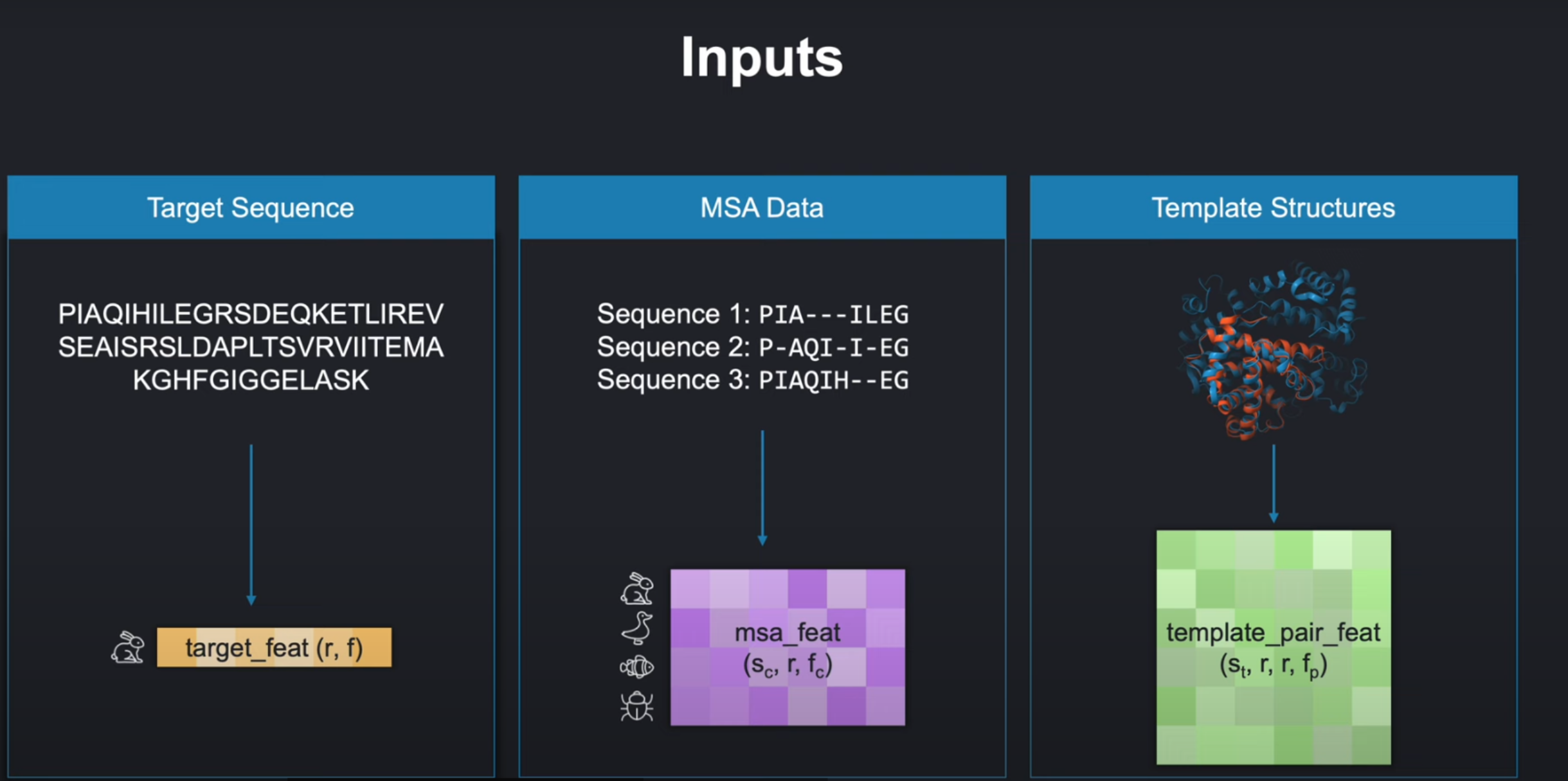
基于现有的蛋白质结构数据。AlphaFold选用了以下三种数据作为输入：

1. 目标氨基酸序列（ amino acid sequence ）
   原始表示形式为字符串，每个字符代表20种氨基酸种的其中一种。氨基酸序列本身也是蛋白质的一级结构。
   我们也就是要预测这个目标氨基酸序列对应的三级结构！

基于蛋白质的进化史，即 基于"进化保守反映结构约束"的生物学原理，还选用了以下两种数据：

2. 多序列比对数据（ multiple sequence alignment data /MSA data ）
   是一组蛋白质序列，它们来自其他不同的生物体(organisms)，但是与我们目标序列高度相似，这也就意味着这些序列有可能起源于相同的祖先。使用这些序列，我们可以获取进化信息，从进行信息种去反应未知的蛋白质结构。

3. 蛋白质三维结构/模板结构（ 3D structure of so called templates ）
   和目标蛋白质相似，但是三维结构已经确定的蛋白质。采样这些蛋白质的三维结构数据表示，也成为模板（templates）。在过去，这一直是与蛋白质结构预测最相关的数据。
   但是很有趣的是，即使AlphaFold并没有使用这些template stack作为输入（特别是当MSA数据足够的多样化且提供了丰富的进化信息时候），也可以达到很好的预测。这也意味着AlphaFold并不需要模板数据作为输入。我们也不会对其进行讲解和代码实现。

2. Datapipline结构介绍

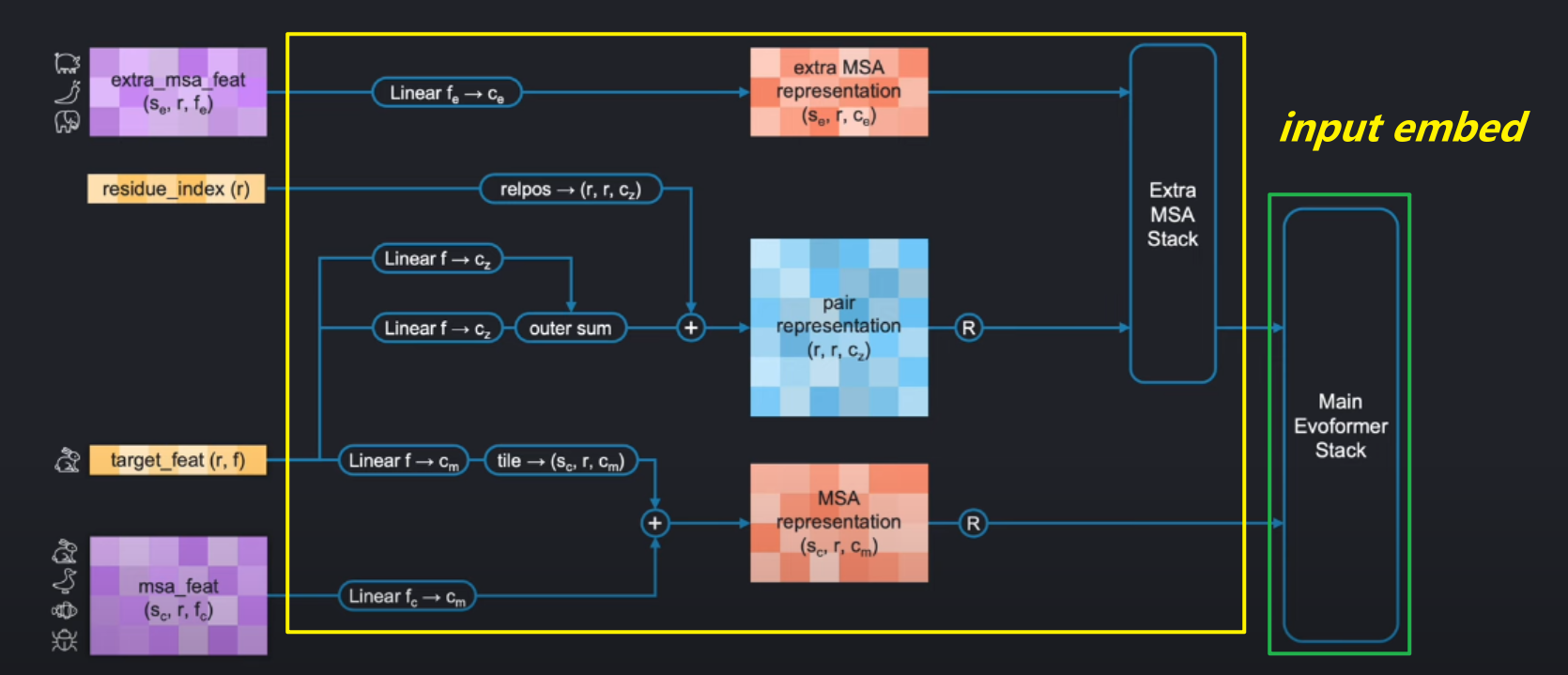
如下图Input Feature Embedding的网络结构所示。在左侧的输入都构建好之后，它们经过输入编码器(input embedder）进行编码。

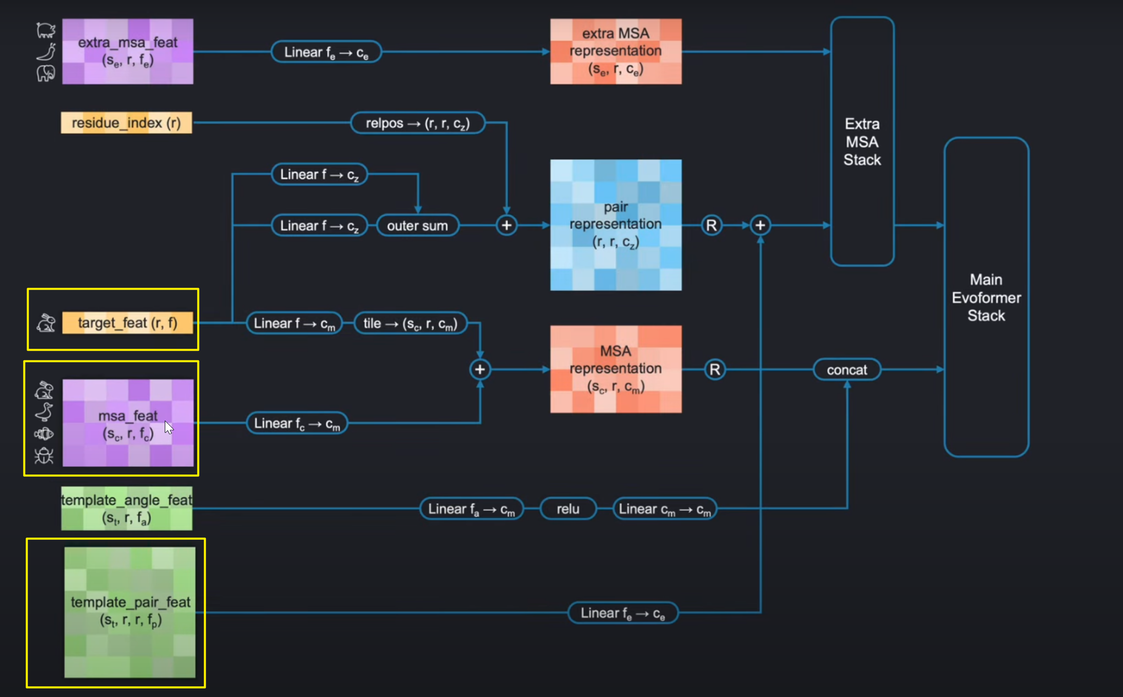
上文说到这里我们不需要考虑template stack，那么整个input pipeline如下：
input embedding and the evoformer stack的实现我们将在接下来的博客进行讲解。这里，我们将实现最左边的四个输入。

其中以下两个很容易理解、确定和实现：

1. Residue_index，就是表示每个氨基酸的索引， range from 0 to r-1，用作后面Evoformerd的位置编码（position encoding)，shape = (r,)，r是氨基酸个数
2. target_feat ：目标氨基酸序列的每个位置氨基酸的独热编码。形状为(r,f) = (r,21)。21代表20个已知氨基酸+1个未知氨基酸。组成长度为21的独热编码。

构建图上剩余的两个msa编码就会复杂一些：

3. extra_msa_feat
4. msa_feat

这两个输入数据都是基于msa的，在这之前，我们需要先了解一下，什么是msa?

4. MSA（多序列比对）基础介绍

蛋白质就是氨基酸组成的序列。我们可以从蛋白质的进化史种提取到很多信息。

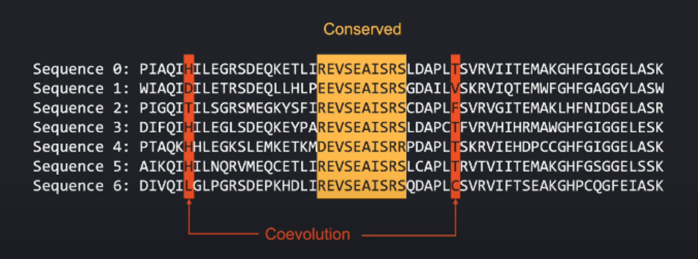
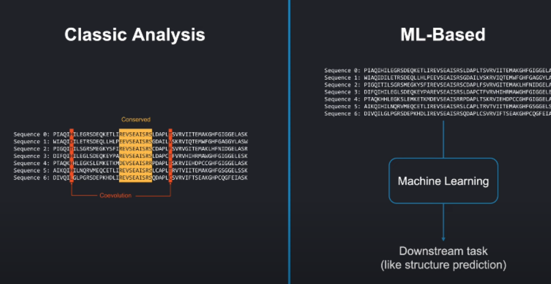
比如，我们可以看在不同的蛋白质种，某个区域是否是高度保守的（Highly conserved)或变化很大。

(1) 保守性（Conservation）分析

• 高度保守区域：

  • 表现：在进化过程中几乎不变的氨基酸位置
  • 意义：通常对应结构或功能核心（如酶活性位点、蛋白质相互作用界面）。
    • 例子：ATP结合位点的GXGXXG模式在激酶中高度保守。

• 低保守区域：

  • 表现：频繁变异的氨基酸位置（如位置4的Ser/Thr/Ala）。
  • 意义：可能是**柔性环区（loops）**或对功能非关键的区域。

(2) 共进化（Coevolution）信号

• 现象：某些氨基酸对会协同突变（一个位置突变，另一位置随之突变）。
• 意义：暗示这些残基在3D空间中物理接近或功能耦合。

进化特征	结构关联	功能关联
高保守残基	核心疏水区、稳定折叠	催化位点、结合位点
低保守区域	表面环区、柔性linker	物种特异性功能适配
共进化残基对	空间邻近（<8Å）	变构调节、信号传递

生物序列分析方法的重大变革——从过去依赖人工设计的显式计算转向数据驱动的机器学习模型

1. 传统方法（Explicit Calculations）

典型技术

• 保守性计算：基于序列比对计算位置熵（如Shannon熵）
• 共进化分析：直接耦合分析（DCA）、互信息（MI）
• 物理势函数：Rosetta中的能量项（如疏水势、氢键势）

局限性

• 浅层模式：只能捕捉预设的简单统计关系（如两两残基耦合）
• 手工特征工程：依赖领域专家设计算法（如定义"保守性阈值=0.8"）
• 任务专用性：换一个新问题（如预测别构效应）需重新设计流程

2. 现代机器学习方法

核心优势

• 深度关联挖掘：自动学习序列中的高阶、非线性模式
  • 例如：同时捕捉残基A↔B↔C的协同约束，而传统方法只能分析A↔B或B↔C
• 端到端学习：直接从原始数据（如MSA）预测结构，无需手动设计中间特征
• 通用性：同一模型架构可适应不同任务（如结构预测、功能注释）

AlphaFold的实现

1. 输入处理：
   • 原始MSA → Evoformer模块自动学习共进化模式
   • 不再需要人工计算DCA矩阵
2. 结构建模：
   • 通过几何注意力（Geometric Attention）直接输出原子坐标
   • 替代了传统基于片段组装+能量最小化的流程

知道进化历史对蛋白质的结构预测很有用，进化历史从MSA数据分析而来，那第一步就是要和目标序列进行比对，找到那些和目标序列相似的序列。

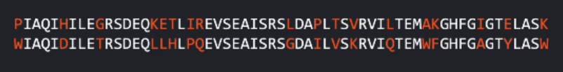
因为蛋白质序列在进化过程中可能有替换substitution、插入insertion或删除deletion，这意味着我们不能一个一个氨基酸比较（ compare positions pointwise）。

比如下面这个序列在白色氨基酸序列都是相同的，整个序列整体上序列结构十分相似。

但是当我们引入/添加一个新的氨基酸时，会导致错位，大部分序列都不匹配了。

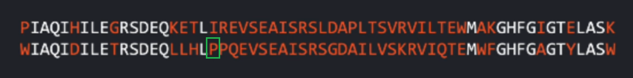
所以，为了让序列尽可能对齐"alignment"，尽可能多的体现出不同蛋白质之间的共同进化的信息。我们需要评估哪些地方有插入和删除。我们允许我们的算法能够在特点位置插入一个-：gap token，表示和目标序列相比这里需要一个插入来与其尽可能好的对齐（ align the sequences as best as it can）

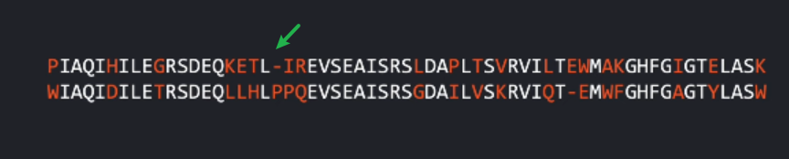
这个比对序列进行对齐的过程主要由 Needlemann-Wunsch 算法完成。Needleman - Wunsch 算法是一种用于生物信息学中进行序列比对的经典动态规划算法，由美国科学家 Needleman 和 Wunsch 在 1970 年提出。该算法主要用于比较两个生物序列（如 DNA、RNA 或蛋白质序列）的相似性，通过在序列中插入空格（gap）来实现最佳的比对，使得相似的区域能够尽可能地对齐，从而推断它们之间的进化关系、功能相似性等。（这里我们不对算法细节进行探讨）

核心问题：序列数据库的庞大规模

1. 内存需求：

   • 主流蛋白质序列数据库（如UniRef、BFD）包含数十亿条序列，加载到内存中需要约 70GB RAM。
   • 对比硬件限制：消费级电脑通常只有16-32GB内存，服务器可能配备128-256GB。

2. 计算成本来源：

   • 搜索对齐：在庞大数据库中查找同源序列（如HHblits/JackHMMER）需要：
     • 扫描所有序列
     • 计算序列相似性
     • 构建多序列比对（MSA）
   • 实时处理：AlphaFold运行时的MSA生成阶段占用了大部分计算时间和内存

组件	内存占用示例	说明
序列数据	UniRef50: ~30GB	压缩存储的序列文本
索引结构	~20GB	加速序列搜索的哈希表/Bloom过滤器
中间比对结果	单个MSA: 100MB-1GB	存储序列比对中的匹配/缺口信息

解决方案：预计算对齐（Precomputed Alignments）

1. ColabFold的实践：

   • 提供预生成的MSA文件（如.a3m格式），跳过实时数据库搜索。
   • 用户可直接下载包含以下内容的压缩包：

     target_sequence.a3m      # 多序列比对文件
     target_sequence.pdb      # 预测结构
     

2. 优势：

   • 内存效率：只需加载单个MSA文件（通常<1GB）
   • 速度提升：避免耗时的序列搜索（从小时级缩短到分钟级）
   • 硬件普适性：可在消费级设备上运行

解释.a3m文件格式：

无论如何，我们最终得到的具有和目标序列对齐的序列比对数据的.a3m文件如下：

整个文件采用交替行的结构，每条序列数据包括两行：>开头的评分数据和紧接着的序列行。第一条序列用101标识，它是目标序列也是query sequence。整个.a3m文件无冗余元数据：仅包含从输入序列通过算法生成的同源序列，不附带实验条件、物种分类等额外信息。

ColabFold的默认行为

• 输入处理：当用户未提供自定义序列时，自动使用大肠杆菌互变异构酶（E. coli Tautomerase）作为示例：

  # ColabFold的默认序列（UniProt P0A6K5）
  DEFAULT_SEQUENCE = "PIAQIHILEGRSDEQKETLIREVSEAISRSLDAPLTSVRVIITEMAKGHFGIGGELASK"
  

• MSA生成：调用MMseqs2快速搜索UniRef/环境数据库，输出精简的.a3m文件。

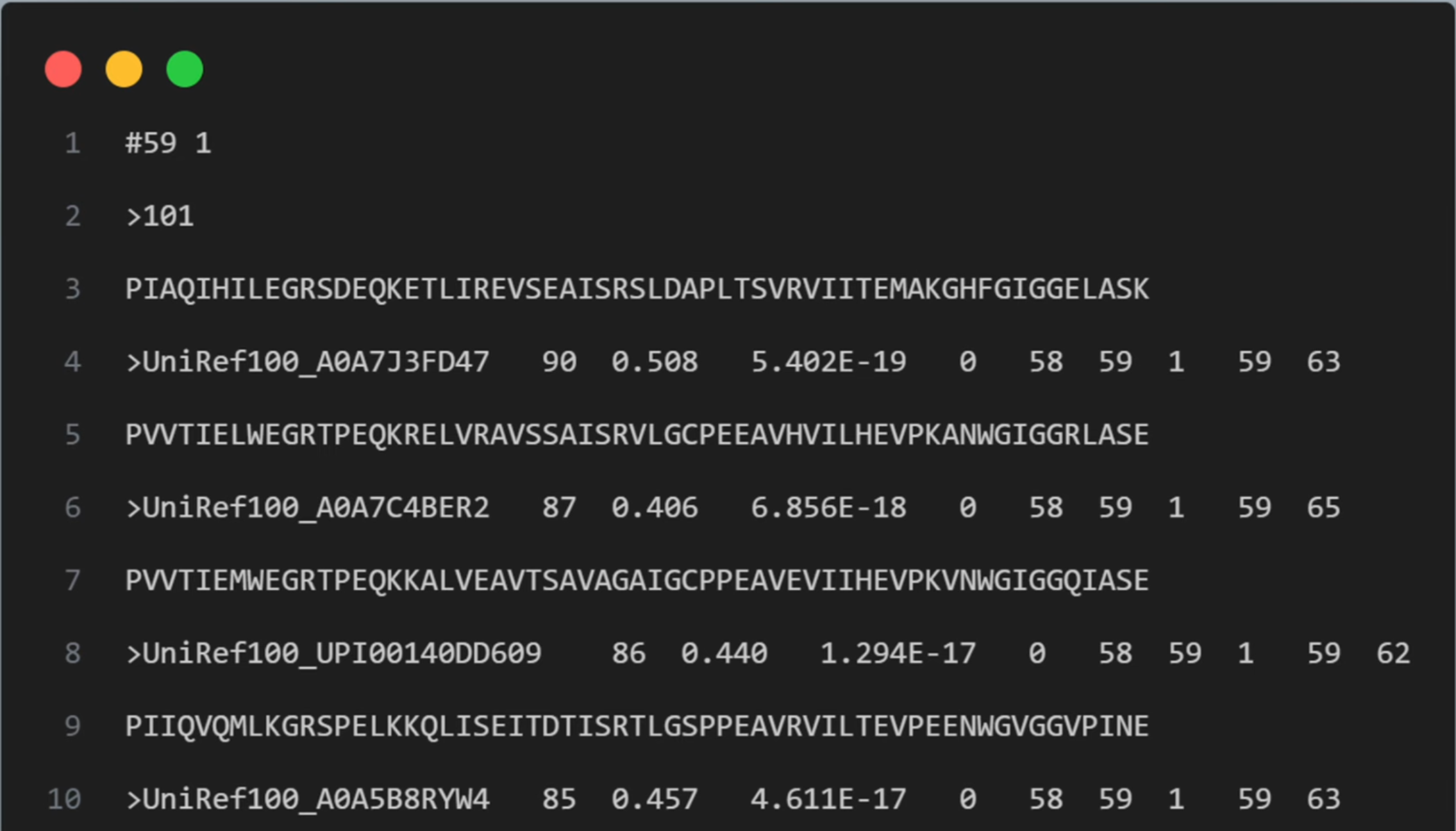
文件结构解析：

1. 第一行 #59 1:
   • #59 表示比对中包含的序列数量(59条)
   • 1 表示第一个序列是查询序列(query sequence)
2. 查询序列部分:

   >101
   PIAQIHILEGRSDEQKETLIREVSEAISRSLDAPLTSVRVIITEMAKGHFGIGGELASK
   

   • >101 是查询序列的标识符
   • 后面是查询序列的氨基酸序列
3. 比对序列部分:
   每个比对序列有以下格式:

   >UniRef100_A0A7J3FD47    90    0.508    5.402E-19    0    58    59    1    59    63
   PVVTIELWEGRTPEQKRELVRAVSSAISRVLGCPEEAVHVILHEVPKANWGIGGRLASE
   

   • 序列头信息(以>开头)包含多个字段:
     1. 序列ID(如UniRef100_A0A7J3FD47)
     2. 序列与查询序列的相似度百分比(90)
     3. 序列覆盖度(0.508)
     4. E-value值(5.402E-19)
     5. 其他比对统计信息
   • 然后是比对后的序列，可能与查询序列长度相同或包含gap(-)

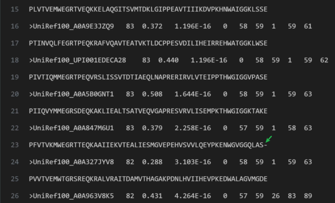
继续往下，在23行，我们第一个看到了gap token:-。它在序列的末尾，代表目标序列在此位置和当前序列相比有一个插入，所以在当前序列使用-占位。

继续看到 393行,我们第一次看到了 deletion: 是氨基酸 glycine, glutamine and glycine, 它们用小写字符表示为 gqg，代表目标序列在此位置没有这几个氨基酸。

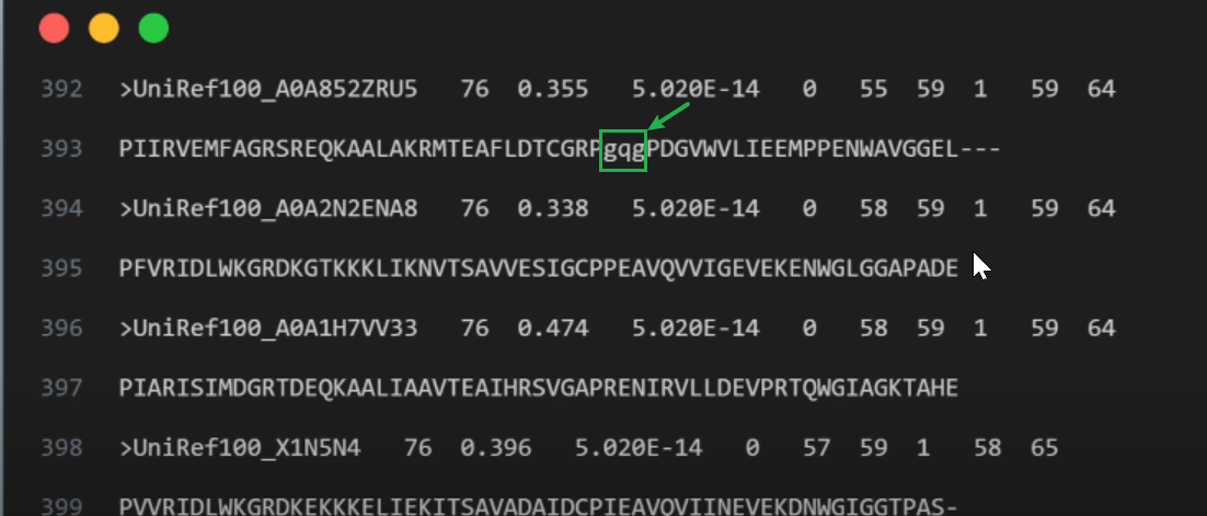
注意当我们谈论到插入和删除时候，我们其实不能真的说在此有插入或者删除，因为我们其实并不知道进化的历史（evolutionary history. ）。如果我们的目标序列比同源的被比较的序列更老，那么插入和删除就是反过来了。不过在这里，我们规定，说到插入和删除，是指从同源序列到目标序列之间的变化。

.a3m多序列比对结果文件在AlphaFold蛋白质结构预测的角色：

5. 特征提取步骤⭐

得到MSA文件后，我们可以从种进行特征提取两类数据：

1. the types of amino acids 氨基酸类型：我们可以知道每个序列每个位置上的氨基酸类型。将其中一部分进行独热编码，其他的一部分序列进行独热编码后取平均值。
2. positions and number of deletions 被删除氨基酸的位置和数量信息：我们可以知道序列种的哪些氨基酸是被删除以及有多少数量。

5.1 初始处理

第一步，统计每个残基左侧的删除数量：

对于所有的氨基酸序列，我们需要找到所有小写字母，它们表示deletions。如何我们计算当前氨基酸的左部有多少deletions，作为当前位置氨基酸的deletion count（如下图）。

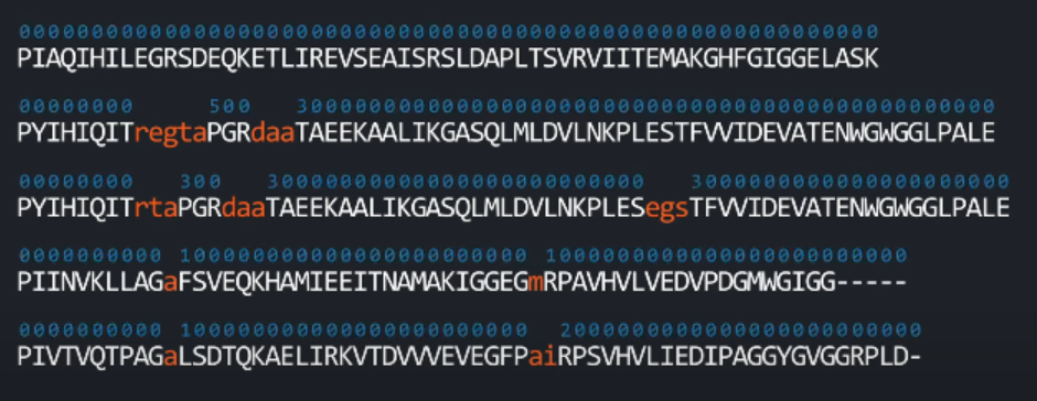
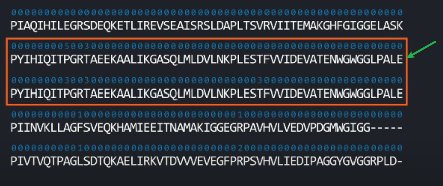
然后，我们删除小写字母，只保留deletion的数量信息：

删除之后，可以看到，包括-在内，所有的同源序列和目标需要都具有相同长度（same length

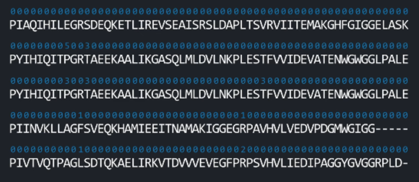
💐note：AlphaFold只使用在删除后唯一的序列，所以如果删除后有序列相同，我们只使用第一个序列。

对序列进行one-hot编码(22类：20氨基酸+未知+gap)，并得到target-feat,shape:(r,21)

我们得到删除之后的序列（without-deletions），对其进行独热编码，每个位置的氨基酸有22类（The 20 amino acids and the unknown and gap tokens）。这些序列同时包括了第一条序列（也就是目标序列），它将独自作one-hot编码，每个位置的氨基酸有21类(20氨基酸+未知），这条序列也将构成模型输入的特征： target_feat.

计算每个位置氨基酸的分布(取one-hot编码的均值)：

经过duress编码后的序列的形状为：(N_seq, N_res, 22)。在此基础上，我们需要另外计算在同一位置的不同氨基酸之间的分布。这个分布将被用为后续步骤中氨基酸的重采样resample 。

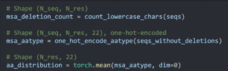
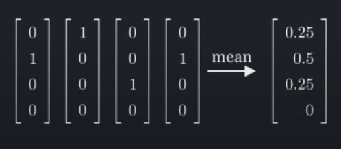
对于aa_distribution的解释：它计算每条序列在同一位置的氨基酸的分布。我们可以把每个氨基酸位置的读热编码的取值表示对这个位置氨基酸的投票。将其加起来求平均可以求得氨基酸在此位置的分布（过程如下图）。

代码实现：

def initial_data_from_seqs(seqs):"""Processes raw sequences from an A3M file to extract initial feature representations.Args:seqs: A list of amino acid sequences loaded from the A3M file. Sequences are represented with single-letter amino acid codes.Lowercase letters represent deletions.Returns:A dictionary containing:* msa_aatype: A PyTorch tensor of one-hot encoded amino acid sequencesof shape (N_seq, N_res, 22), where N_seq is the number of unique sequences (with deletions removed) and N_res is the length of the sequences. The dimension 22 corresponds to the 20 amino acids, an unknown amino acid token, and a gap token. * msa_deletion_count: A tensor of shape (N_seq, N_res) where each element represents the number of deletions occurring before the corresponding residue in the MSA.* aa_distribution: A tensor of shape (N_res, 22) containing the overall amino acid distribution at each residue position across the MSA.  """unique_seqs = Nonedeletion_count_matrix = Noneaa_distribution = None########################################################################### TODO:                                                                  ## 1. Calculate the 'deletion_count_matrix':                              ##    * Initialize an empty list of lists to store deletion counts.       ##    * Iterate through the sequences in 'seqs':                          ##       * Create a list to track deletions for the current sequence.     ##       * Iterate through letters, counting lowercase letters            ##         as deletions.                                                  ##       * Append the deletion count list to the main                     ##         'deletion_count_matrix' only if the sequence                   # #         (after removing deletions) has not been seen before.           ##    * Convert 'deletion_count_matrix' into a PyTorch tensor.            ## 2. Identify 'unique_seqs':                                             ##    * Create an empty list to store unique sequences.                   ##    * Iterate through the sequences in 'seqs':                          ##       * Remove lowercase letters (deletions) from the sequence.        ##       * If the sequence (without deletions) is not already in the      ##         'unique_seqs' list, add it.                                    ##    * Apply the `onehot_encode_aa_type` function to each sequence       ##      in 'unique_seqs' to get a tensor of shape (N_seq, N_res, 22)      ##      representing the one-hot encoded amino acids.                     ## 3. Compute 'aa_distribution':                                          ##    * Average the one-hot encoded 'unique_seqs' tensor across the       ##      first dimension (representing sequences) to calculate the         ##      amino acid distribution.                                          ###########################################################################deletion_count_matrix = []unique_seqs = []for seq in seqs:deletion_count_list = []deletion_counter = 0for letter in seq:if letter.islower():deletion_counter += 1else:deletion_count_list.append(deletion_counter)deletion_counter=0seq_without_deletion = re.sub('[a-z]', '', seq)if seq_without_deletion in unique_seqs:continueunique_seqs.append(seq_without_deletion)deletion_count_matrix.append(deletion_count_list)unique_seqs = torch.stack([onehot_encode_aa_type(seq, include_gap_token=True) for seq in unique_seqs], dim=0)unique_seqs = unique_seqs.float()deletion_count_matrix = torch.tensor(deletion_count_matrix).float()aa_distribution = unique_seqs.float().mean(dim=0)########################################################################### END OF YOUR CODE                                                       ###########################################################################return { 'msa_aatype': unique_seqs, 'msa_deletion_count': deletion_count_matrix, 'aa_distribution': aa_distribution}

经过上述对.asm文件的初始处理，我们得到了

• msa_aatype;shape(N_seq,N_res,22]、
• msa_deletion_count;shape(N_seq,N_res)、
• aa_distribution;shape(N_res,22)

基于这个，我们正式开始以下五个步骤的讲解AlphaFold中的特征提取部分：

1. 首先，AlphaFold会随机选择一些数量的序列作为“聚类中心”。这些序列会被直接作为特征，而其他没有被选中的序列作为“extra" sequences，只为每一cluster的均值作出贡献。

2. 完成聚类中心的选择后，作为聚类中心的这部分序列也会被随机的改变，在论文中被称为’masking’

3. 然后，额外的序列会被分配到那些与之最为相近的聚类中心。

4. deletions的数量会在每一个聚类中被平均

5. 最终，这些特征会被stack(堆叠）来作为full msa_feat特征

5.2 聚类中心选择

首先，我们会随机的选取一定数量的序列作为聚类中心（cluster centers)，这之中会始终包括目标序列作为第一个中心（always including the target sequence as the first center.）。

对于每个聚类中心，我们分别提取它的 deletions and amino acids ，对于其他的序列，我们直接对其进行平均。

关键特性

特性	说明
非均匀分布	簇中心是随机选择的，不保证空间均匀覆盖
目标序列必选	索引0强制包含，确保目标序列信息不被丢失
固定数量(512)	平衡计算成本与表征能力（实验验证的折中点）
Extra MSA的作用	未被选中的序列仍用于共进化信号提取，但计算开销更低

生物学合理性
虽然看似简单，但这种策略有效是因为：

1. MSA冗余性：同源序列本身具有相似性，随机采样大概率覆盖主要变异模式
2. 注意力机制补偿：Evoformer的self-attention能自动加权重要序列
3. 计算效率优先：避免昂贵的聚类计算（如k-means需O(N^2)距离矩阵）

示例数据流
假设MSA有10,000条序列：

1. 生成随机排列：[5832, 1241, 9999, ..., 42]
2. 添加目标序列：[0, 5832, 1241, ..., 42]
3. 选取前512个：[0, 5832, 1241, ..., 511th] → 簇中心
4. 剩余9,488条 → Extra MSA

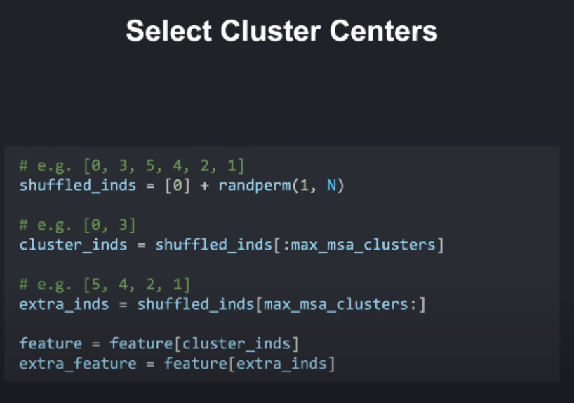
代码实现：

def select_cluster_centers(features, max_msa_clusters=512, seed=None):"""Selects representative sequences as cluster centers from the MSA to  reduce redundancy.Args:features: A dictionary containing feature representations of the MSA.max_msa_clusters: The maximum number of cluster centers to select.seed: An optional integer seed for the random number generator. Use this to ensure reproducibility.Modifies:The 'features' dictionary in-place by:* Updating the 'msa_aatype' and 'msa_deletion_count' features to contain data for the cluster centers only.  * Adding 'extra_msa_aatype' and 'extra_msa_deletion_count' featuresto hold the data for the remaining (non-center) sequences. """N_seq, N_res = features['msa_aatype'].shape[:2]MSA_FEATURE_NAMES = ['msa_aatype', 'msa_deletion_count']max_msa_clusters = min(max_msa_clusters, N_seq)gen = Noneif seed is not None:gen = torch.Generator(features['msa_aatype'].device)gen.manual_seed(seed)########################################################################### TODO:# 1. **Implement Shuffling:**#      * Use  `torch.randperm(N_seq - 1)` with the provided  `gen` (random number generator) #        to shuffle the indices from 1 to (N_seq - 1). Ensure reproducibility if the seed is not None.#      * Prepend a 0 to the shuffled indices to include the first sequence.# 2. **Split Features:**#      * Using the shuffled indices,  split the MSA feature representations (`msa_aatype` and#        `msa_deletion_count`) into two sets:#          *  The first `max_msa_clusters` sequences will be the cluster centers.#          *  The remaining sequences will be stored with keys prefixed by  'extra_'. ##########################################################################shuffled = torch.randperm(N_seq-1, generator=gen) + 1shuffled = torch.cat((torch.tensor([0]), shuffled), dim=0)for key in MSA_FEATURE_NAMES:extra_key = f'extra_{key}'value = features[key]features[extra_key] = value[shuffled[max_msa_clusters:]]features[key] = value[shuffled[:max_msa_clusters]]########################################################################### END OF YOUR CODE                                                       ###########################################################################return features

5.3 聚类掩码(Cluster Masking)

接下来就是对聚类中心的序列的部分氨基酸（15%）进行聚类掩码，页就是对其进行改动。

用于增强模型鲁棒性的序列掩码正则化技术，其核心思想是通过随机扰动簇中心序列，使模型能够学习更稳健的特征表示。

💐分步掩码流程：

1. 初始选择（15%概率）：

   • 每个簇中心的每个氨基酸位置有15%的概率被选中进行可能的替换

2. 替换策略（对选中位置）：

   替换类型	概率	说明
   随机氨基酸替换	10%	从20种标准氨基酸中均匀采样
   基于MSA分布的替换	10%	根据该位置在MSA中的氨基酸频率分布采样
   保持原氨基酸	10%	即使被选中也不改变
   掩码标记（[MASK]）替换	70%	用特殊token替换，模拟数据缺失场景

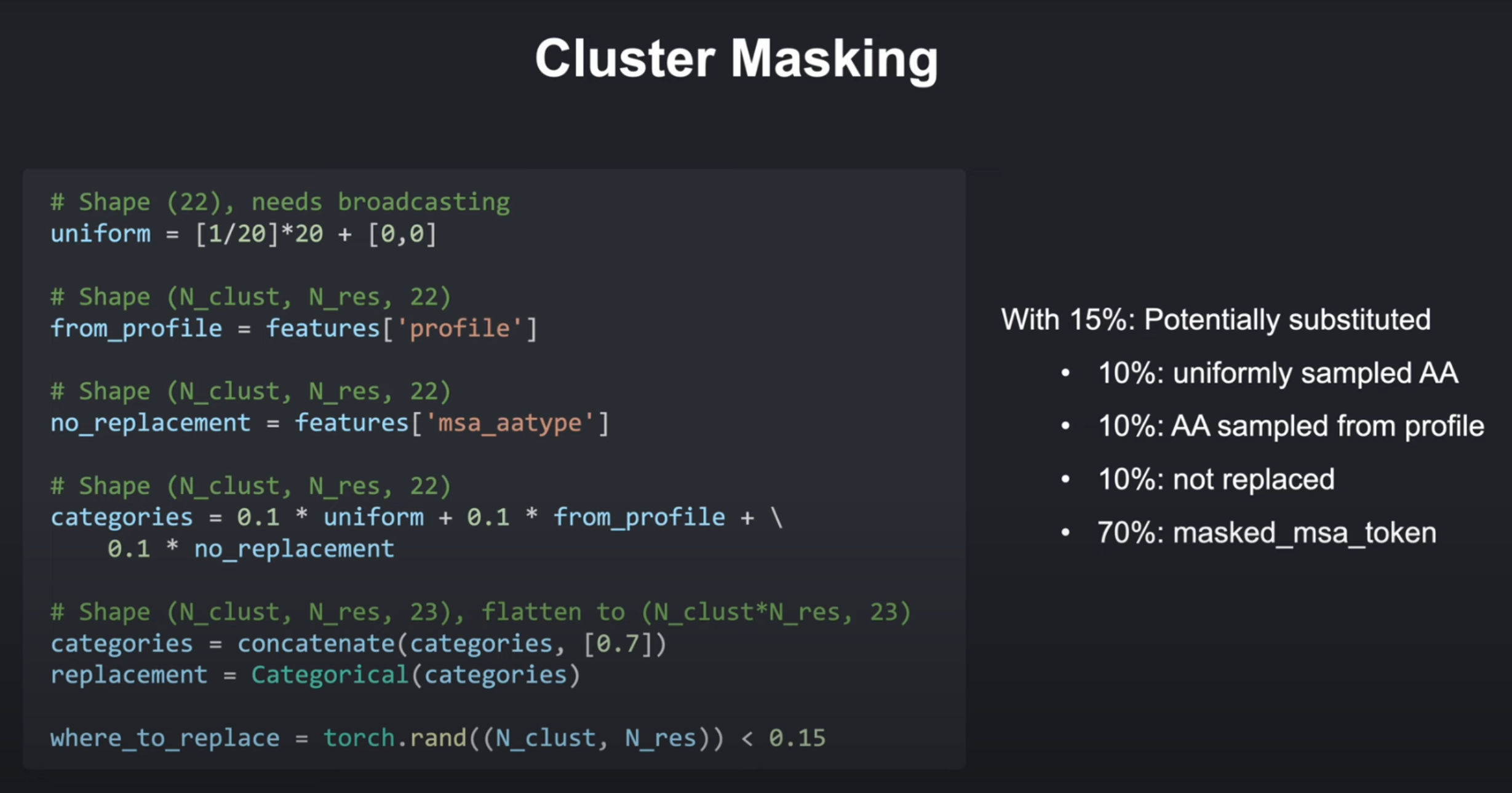
代码实现

def mask_cluster_centers(features, mask_probability=0.15, seed=None):"""Introduces random masking in the cluster center sequences for data augmentation.This function modifies the 'msa_aatype' feature within the 'features' dictionary to improve model robustness in the presence of noisy or missing input data.  Masking is inspired by the AlphaFold architecture.Args:features: A dictionary containing feature representations of the MSA. It is assumedthat cluster centers have already been selected.mask_probability: The probability of masking out an individual amino acid in a cluster center sequence.seed: An optional integer seed for the random number generator. Use this to ensure reproducibility.Modifies:The 'features' dictionary in-place by:* Updating the 'msa_aatype' feature with masked-out tokens as well as possible replacements based on defined probabilities. * Creating a copy of the original 'msa_aatype' feature with the key 'true_msa_aatype'. """N_clust, N_res = features['msa_aatype'].shape[:2]N_aa_categories = 23 # 20 Amino Acids, Unknown AA, Gap, masked_msa_tokenodds = { # 定义四种替换路径的权重'uniform_replacement': 0.1,  # 随机替换'replacement_from_distribution': 0.1, # MSA分布替换'no_replacement': 0.1, # 保持'masked_out': 0.7, # 特殊掩码}gen = Noneif seed is not None:gen = torch.Generator(features['msa_aatype'].device)gen.manual_seed(seed)torch.manual_seed(seed)########################################################################### TODO:# 1. **Select Modification Candidates:**#      * Generate a random mask (tensor of shape (N_clust, N_res) ) where each element is a #        random number between 0 and 1. #      * Select elements where the random number is less than the `mask_probability` for potential modification.# 2. **Replacement Logic:**#      * Create tensors to represent substitution probabilities:#          * `uniform_replacement`: Shape (22,) #             - Set the first 20 elements (amino acids) to `1/20 * odds['uniform_replacement']`.#             - Set the last 2 elements (unknown AA and gap) to 0.#          * `replacement_from_distribution`: Shape (N_res, 22), calculated from 'features['aa_distribution]'. Scale by `odds['replacement_from_distribution']`#          *  `no_replacement`: Shape (N_clust, N_res, 22), use the existing 'features['msa_aatype']' tensor and scale by `odds['no_replacement']`.#          * `masked_out`: Shape (N_clust, N_res, 1), all elements are `odds['masked_out']`.#      * **Sum** the first three tensors, then **concatenate** with `masked_out` along the last dimension.  This creates 'categories_with_mask_token' of shape (N_clust, N_res, 23)#      * Flatten the first two dimensions of 'categories_with_mask_token' for sampling.#      * Use  `torch.distributions.Categorical` and the flattened 'categories_with_mask_token' tensor to #        probabilistically determine replacements for the selected residues. #      * Reshape the sampled replacements back to (N_clust, N_res).# 3. **Preserve Original Data:**#      * Create a copy of the original 'msa_aatype' data under the key 'true_msa_atype'.# 4. **Apply Masking:**#      * Update the 'msa_aatype' tensor, but *only* for the elements selected in step 1 for modification, with the sampled replacements.  Leave other elements unchanged. ########################################################################### uniform_replacement has shape (22,) uniform_replacement = torch.tensor([1/20]*20+[0,0]) * odds['uniform_replacement']# replacement_from_distribution has shape (N_res, 22)replacement_from_distribution = features['aa_distribution'] * odds['replacement_from_distribution']# no_replacement has shape (N_clust, N_res, 22)no_replacement = features['msa_aatype'] * odds['no_replacement']# masked_out has shape (N_clust, N_res, 1)masked_out = torch.ones((N_clust, N_res, 1)) * odds['masked_out']uniform_replacement = uniform_replacement[None, None, ...].broadcast_to(no_replacement.shape)replacement_from_distribution = replacement_from_distribution[None, ...].broadcast_to(no_replacement.shape)# 计算联合概率分布categories_without_mask_token = uniform_replacement + replacement_from_distribution + no_replacement# (N_clust, N_res, 22) categories_with_mask_token = torch.cat((categories_without_mask_token, masked_out), dim=-1)# (N_clust, N_res, 22) + （N_clust, N_res, 1) = (N_clust, N_res, 23)categories_with_mask_token = categories_with_mask_token.reshape(-1, N_aa_categories) # (N_clust * N_res, 23)replace_with = torch.distributions.Categorical(categories_with_mask_token).sample() # 采样replace_with = nn.functional.one_hot(replace_with, num_classes=N_aa_categories)replace_with = replace_with.reshape(N_clust, N_res, N_aa_categories)replace_with = replace_with.float()# 掩码replace_mask = torch.rand((N_clust, N_res), generator=gen) < mask_probabilityfeatures['true_msa_aatype'] = features['msa_aatype'].clone()aatype_padding = torch.zeros((N_clust, N_res, 1))features['msa_aatype'] = torch.cat((features['msa_aatype'], aatype_padding), dim=-1)features['msa_aatype'][replace_mask] = replace_with[replace_mask]########################################################################### END OF YOUR CODE                                                       ###########################################################################return features

5.4 聚类分配

当对特征中心进行掩码之后，额外的氨基酸序列将被分配到这些聚类中心。通过计算有多少氨基酸和聚类中心序列中的氨基酸相似。这也被两条序列的汉明距离。（注意，我们只计算氨基酸，如果是gap则不考虑）。

每条额外的序列会被分配给与之最相似的聚类中心。这可以用argmax来评估。另外我们会统计每个聚类中心被分配了多少个序列（cluster-size)，会用在下面计算聚类平均。

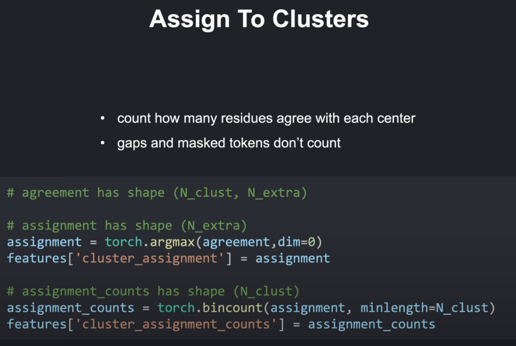
代码实现：

def cluster_assignment(features):"""Assigns sequences in the extra MSA to their closest cluster centers based on Hamming distance.Args:features: A dictionary containing feature representations of the MSA. It is assumed that cluster centers have already been selected.Returns:The updated 'features' dictionary with the following additions:* cluster_assignment:  A tensor of shape (N_extra,) containing the indices of the assigned cluster centers for each extra sequence.* cluster_assignment_counts: A tensor of shape (N_clust,)  where each element indicates the number of extra sequences assigned to a cluster center (excluding the cluster center itself)."""N_clust, N_res = features['msa_aatype'].shape[:2]N_extra = features['extra_msa_aatype'].shape[0]########################################################################### TODO:# 1. **Prepare Features:**#     * Obtain slices of the 'msa_aatype' (shape: N_clust, N_res, 23) and 'extra_msa_aatype' (shape: N_extra, N_res, 22) tensors #       that exclude the  'gap' and 'masked' tokens.  This focuses the calculation on the standard amino acids.# 2. **Calculate Agreement:**#     * Employ broadcasting and tensor operations on the prepared features to efficiently calculate the number of positions where #       the amino acids in each extra sequence agree with those in each cluster center.  The result will be an 'agreement' tensor #       of shape (N_clust, N_extra).  `torch.einsum` can be a useful tool here. # 3. **Assign Clusters:**#     * Use `torch.argmax(agreement, dim=0)` to find the cluster center index with the highest agreement (lowest Hamming distance) for each extra sequence. # 4. **Compute Assignment Counts:** #     * Use `torch.bincount` to efficiently calculate the number of extra sequences assigned to each cluster center (excluding #       the cluster center itself).  Ensure you set the `minlength` parameter appropriately.##########################################################################msa_aatype = features['msa_aatype'][...,:21]extra_msa_aatype = features['extra_msa_aatype'][...,:21]agreement = torch.einsum('cra,era->ce', msa_aatype, extra_msa_aatype)assignment = torch.argmax(agreement,dim=0)features['cluster_assignment'] = assignmentassignment_counts = torch.bincount(assignment, minlength=N_clust)features['cluster_assignment_counts'] = assignment_counts########################################################################### END OF YOUR CODE                                                       ###########################################################################return features

5.5 聚类平均

这里，我们会对之前提取的deletion-count和每个位置的

1. 输入数据准备

变量	形状	含义
cluster_features	(N_clust, N_res, C)	初始簇中心特征（含氨基酸分布、缺失计数等）
extra_features	(N_extra, N_res, C)	额外序列的特征
cluster_assignment	(N_extra,)	每个额外序列所属的簇索引（通过汉明距离计算得到）
cluster_assignment_count	(N_clust,)	每个簇分配到的额外序列数量（通过bincount得到）

2. 计算步骤分解
(1) 特征累加（Scatter Add）
使用torch.scatter_add将额外序列特征按簇归属累加到簇中心：

# 扩展cluster_assignment形状以匹配extra_features
expanded_assignment = cluster_assignment.view(-1, 1, 1).expand_as(extra_features)  # (N_extra, N_res, C)# 累加操作
cluster_sums = torch.zeros_like(cluster_features)
cluster_sums.scatter_add_(dim=0, index=expanded_assignment, src=extra_features)  # (N_clust, N_res, C)

(2) 计算平均值
由于平均值需包含簇中心本身，分母为assignment_counts + 1：

# 扩展计数形状以匹配特征维度
counts = (cluster_assignment_count + 1).view(-1, 1, 1)  # (N_clust, 1, 1)# 计算平均特征
cluster_avg = cluster_sums / counts  # (N_clust, N_res, C)

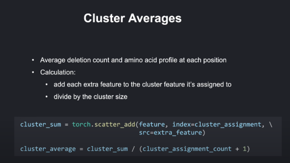
完整代码：

def cluster_average(feature, extra_feature, cluster_assignment, cluster_assignment_count):"""Calculates the average representation of each cluster center by aggregating features from the assigned extra sequences.Args:feature: A tensor containing feature representations for the cluster centers.Shape: (N_clust, N_res, *)extra_feature: A tensor containing feature representations for extra sequences.Shape: (N_extra, N_res, *).  The trailing dimensions (*) must be smaller or equal to those of the 'feature' tensor.cluster_assignment: A tensor indicating the cluster assignment of each extra sequence.Shape: (N_extra,)cluster_assignment_count: A tensor containing the number of extra sequences assigned to each cluster center.Shape: (N_clust,)Returns:A tensor containing the average feature representation for each cluster. Shape: (N_clust, N_res, *) """N_clust, N_res = feature.shape[:2]N_extra = extra_feature.shape[0]########################################################################### TODO:# 1. **Prepare for Accumulation:**#     * Broadcast the `cluster_assignment` tensor to have the same shape as `extra_feature`.#     This is necessary for compatibility with `torch.scatter_add`.# 2. **Accumulate Features:**#     * Use `torch.scatter_add` to efficiently sum (or accumulate) the `extra_feature` values  for each cluster.  The broadcasted `cluster_assignment` tensor will define the grouping. # 3. **Calculate Averages:**#     * Divide the accumulated features by the `cluster_assignment_count` + 1 to obtain the average feature representations for each cluster. ##########################################################################unsqueezed_extra_shape = (N_extra,) + (1,) * (extra_feature.dim()-1)unsqueezed_cluster_shape = (N_clust,) + (1,) * (feature.dim()-1)cluster_assignment = cluster_assignment.view(unsqueezed_extra_shape).broadcast_to(extra_feature.shape)cluster_sum = torch.scatter_add(feature, dim=0, index=cluster_assignment, src=extra_feature)cluster_assignment_count = cluster_assignment_count.view(unsqueezed_cluster_shape).broadcast_to(feature.shape)cluster_average = cluster_sum / (cluster_assignment_count + 1)########################################################################### END OF YOUR CODE                                                       ###########################################################################return cluster_average

5.6 特征堆叠

这是最后一次真正的计算。现在，剩下要做的就是收集我们构建的特征并正确堆叠它们。

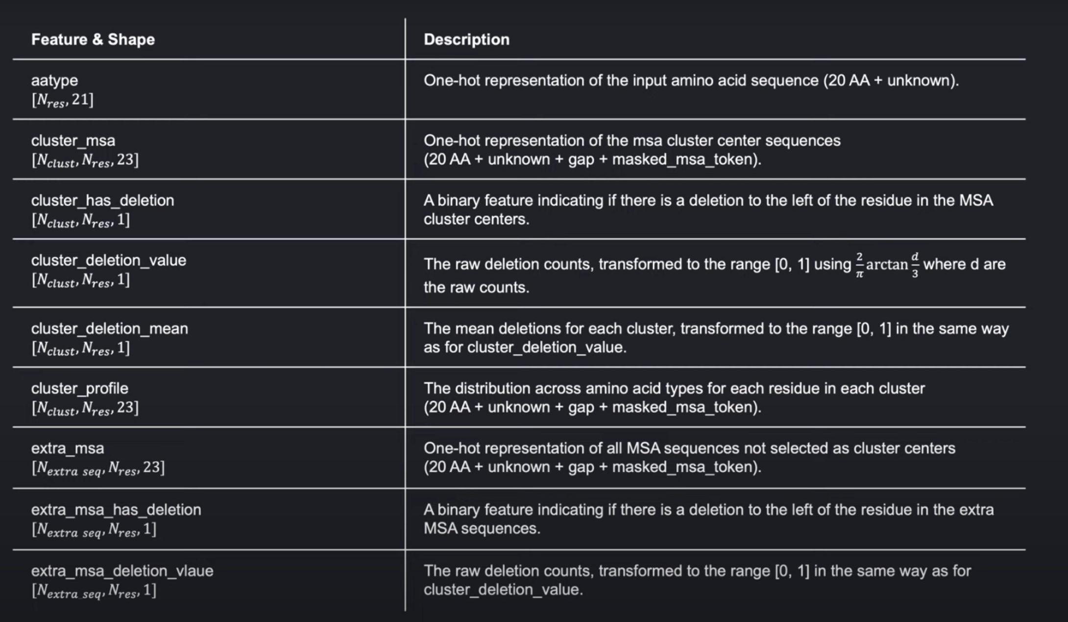
下面这张表格是AlphaFold从.a3m文件构造的所有特征，我们将全部过一遍。

• The feature aatype is a one-hot encoding of the input sequence.

• cluster_msa is the same for all sequences that were selected as cluster centers. Note that we need two additional tokens in the one-hot encoding, for gap tokens and mask tokens.

• The feature cluster_has_deletion is one for every residue in the cluster centers that had a deletion on its left, zero otherwise.

• cluster_deletion_value actually counts the number of deletions on the left of each residue, then normalizes it by 2/pi*arctan(d/3). This maps the values to a range (0, 1), which is better suited as a network input.

• The features extra_msa, extra_msa_has_deletion and extra_msa_deletion_value are identical to the ones for the cluster centers, but calculated for all sequences that were not selected. These features will be used as input through the less complex, memory-friendly Extra MSA Stack.

• For the main input, the extra sequences only contribute as averages for each cluster, by the features cluster_deletion_mean and cluster_profile. They contain just what the names suggest: cluster_deletion_mean is the average number of deletions left to each residue for each sequence in the clusters, normalized to the range [0,1] using arctan again, and cluster_profile is a distribution over the amino acids at each position. Note that the averages also include the cluster centers.

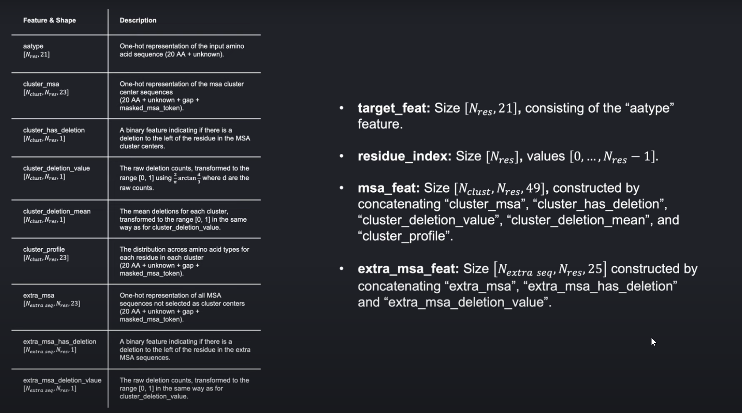
我们上面的步骤其实我们已经得到了那些特征。接下来就是将他们进行处理得到模型的输入 concatenate some of them to get the final inputs:

• The feature ‘target_feat’ is the ‘aatype’ feature.
• The feature ‘residue_index’ is a range of [0, ..., N_res-1], to be used for positional encodings.
• The feature ‘msa_feat’ is constructed by concatenating ‘cluster_msa’, ‘cluster_has_deletion’, ‘cluster_deletion_value’, ‘cluster_deletion_mean’ and ‘cluster_profile’.
• The feature ‘extra_msa'feat’ is constructed by concatenating ‘extra_msa’, ‘extra_msa_has_deletion’ and ‘extra_msa_deletion_value’.
  

注意我们在构建这些输入的时候使用了随机性，尤其是在构建聚类中心的时候还有聚类掩码的时候。

在后面我们会看到AlphaFold会重复作几次这样完整的预测，循环预测positions和其他输出。这些输入构建的步骤会在模型每次推理的时候重新执行，这意味着每次迭代的时候都会有随机性。

–

总结

综上，这就是AlphaFold的特征提取的流程。

从相关的输入数据中进行选择，然后将其转为tensor数据类型是机器学习在新的问题背景下的关键。