乳腺癌识别:双模型融合
本文为为🔗365天深度学习训练营内部文章
原作者:K同学啊
import matplotlib.pyplot as plt
import tensorflow as tf
import warnings as w
w.filterwarnings('ignore')
# 支持中文
plt.rcParams['font.sans-serif'] = ['SimHei']  # 用来正常显示中文标签
plt.rcParams['axes.unicode_minus'] = False  # 用来正常显示负号

import os,PIL,pathlib

#隐藏警告
import warnings
warnings.filterwarnings('ignore')

data_dir = "./J3-data"
data_dir = pathlib.Path(data_dir)

image_count = len(list(data_dir.glob('*/*')))

print("图片数为:",image_count)
图片数为: 13403
batch_size = 64
img_height = 224
img_width = 224

train_ds = tf.keras.preprocessing.image_dataset_from_directory(
    data_dir,
    validation_split=0.3,
    subset="training",
    seed=12,
    image_size=(img_height, img_width),
    batch_size=batch_size)
Found 13403 files belonging to 2 classes. Using 9383 files for training.
val_ds = tf.keras.preprocessing.image_dataset_from_directory(
    data_dir,
    validation_split=0.3,
    subset="validation",
    seed=12,
    image_size=(img_height, img_width),
    batch_size=batch_size)
Found 13403 files belonging to 2 classes. Using 4020 files for validation.
class_names = train_ds.class_names
print(class_names)

for image_batch, labels_batch in train_ds:
    print(image_batch.shape)
    print(labels_batch.shape)
    break

AUTOTUNE = tf.data.AUTOTUNE

def preprocess_image(image,label):
    return (image/255.0,label)

# 归一化处理
train_ds = train_ds.map(preprocess_image, num_parallel_calls=AUTOTUNE)
val_ds   = val_ds.map(preprocess_image, num_parallel_calls=AUTOTUNE)

train_ds = train_ds.cache().shuffle(1000).prefetch(buffer_size=AUTOTUNE)
val_ds   = val_ds.cache().prefetch(buffer_size=AUTOTUNE)

plt.figure(figsize=(15, 10))  # 图形的宽为15高为10

for images, labels in train_ds.take(1):
    for i in range(15):

        ax = plt.subplot(3, 5, i + 1)
        plt.imshow(images[i])
        plt.title(class_names[labels[i]])

        plt.axis("off")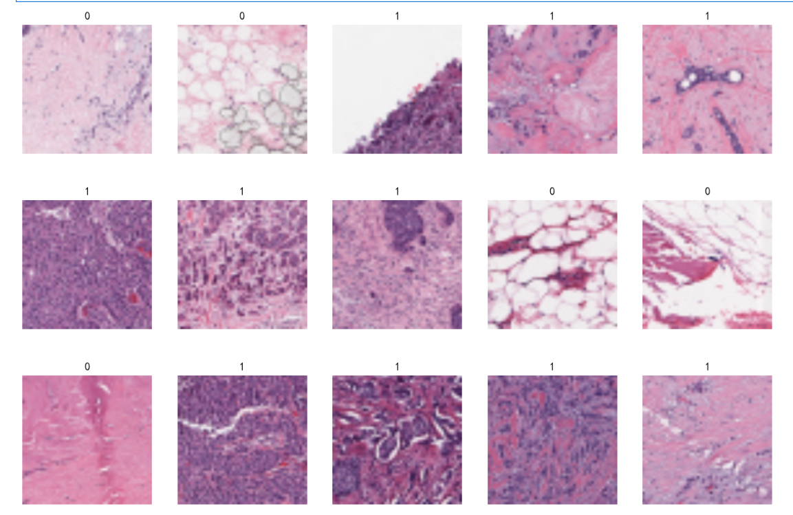
import tensorflow as tf
from tensorflow.keras import layers, models
from tensorflow.keras.applications import ResNet50, DenseNet121
from tensorflow.keras.layers import GlobalAveragePooling2D, Concatenate, Dense, Dropout, BatchNormalization, Multiply, Reshape

# SE-Net 模块
def se_block(input_tensor, ratio=16):
    channels = input_tensor.shape[-1]
    se = GlobalAveragePooling2D()(input_tensor)  # Squeeze
    se = Dense(channels // ratio, activation='relu')(se)
    se = Dense(channels, activation='sigmoid')(se)  # Excitation
    se = Reshape((1, 1, channels))(se)
    return Multiply()([input_tensor, se])  # Scale

# 创建模型
def create_model(input_shape=(224, 224, 3)):
    # 加载预训练的 ResNet50 和 DenseNet121
    resnet_base = ResNet50(weights='imagenet', include_top=False, input_shape=input_shape)
    densenet_base = DenseNet121(weights='imagenet', include_top=False, input_shape=input_shape)

    # 冻结卷积层
    for layer in resnet_base.layers:
        layer.trainable = False
    for layer in densenet_base.layers:
        layer.trainable = False

    # 输入层
    inputs = layers.Input(shape=input_shape)

    # ResNet 分支
    x1 = resnet_base(inputs)
    x1 = BatchNormalization()(x1)  # 添加 BN
    x1 = se_block(x1)  # 添加 SE-Net
    x1 = GlobalAveragePooling2D()(x1)

    # DenseNet 分支
    x2 = densenet_base(inputs)
    x2 = BatchNormalization()(x2)  # 添加 BN
    x2 = se_block(x2)  # 添加 SE-Net
    x2 = GlobalAveragePooling2D()(x2)

    # 拼接特征
    x = Concatenate()([x1, x2])
    x = Dense(256, activation='relu')(x)
    x = BatchNormalization()(x)  # 添加 BN
    x = Dropout(0.5)(x)
    outputs = Dense(num_classes, activation='sigmoid')(x)

    # 构建模型
    model = models.Model(inputs, outputs)
    return model

# 创建并编译模型
num_classes = 2  # 二分类
model = create_model()
model.summary()
Model: "model"
__________________________________________________________________________________________________
Layer (type) Output Shape Param # Connected to
==================================================================================================
input_3 (InputLayer) [(None, 224, 224, 3 0 []
)]
resnet50 (Functional) (None, 7, 7, 2048) 23587712 ['input_3[0][0]']
densenet121 (Functional) (None, 7, 7, 1024) 7037504 ['input_3[0][0]']
batch_normalization (BatchNorm (None, 7, 7, 2048) 8192 ['resnet50[0][0]']
alization)
batch_normalization_1 (BatchNo (None, 7, 7, 1024) 4096 ['densenet121[0][0]']
rmalization)
global_average_pooling2d (Glob (None, 2048) 0 ['batch_normalization[0][0]']
alAveragePooling2D)
global_average_pooling2d_2 (Gl (None, 1024) 0 ['batch_normalization_1[0][0]']
obalAveragePooling2D)
dense (Dense) (None, 128) 262272 ['global_average_pooling2d[0][0]'
]
dense_2 (Dense) (None, 64) 65600 ['global_average_pooling2d_2[0][0
]']
dense_1 (Dense) (None, 2048) 264192 ['dense[0][0]']
dense_3 (Dense) (None, 1024) 66560 ['dense_2[0][0]']
reshape (Reshape) (None, 1, 1, 2048) 0 ['dense_1[0][0]']
reshape_1 (Reshape) (None, 1, 1, 1024) 0 ['dense_3[0][0]']
multiply (Multiply) (None, 7, 7, 2048) 0 ['batch_normalization[0][0]',
'reshape[0][0]']
multiply_1 (Multiply) (None, 7, 7, 1024) 0 ['batch_normalization_1[0][0]',
'reshape_1[0][0]']
global_average_pooling2d_1 (Gl (None, 2048) 0 ['multiply[0][0]']
obalAveragePooling2D)
global_average_pooling2d_3 (Gl (None, 1024) 0 ['multiply_1[0][0]']
obalAveragePooling2D)
concatenate (Concatenate) (None, 3072) 0 ['global_average_pooling2d_1[0][0
]',
'global_average_pooling2d_3[0][0
]']
dense_4 (Dense) (None, 256) 786688 ['concatenate[0][0]']
batch_normalization_2 (BatchNo (None, 256) 1024 ['dense_4[0][0]']
rmalization)
dropout (Dropout) (None, 256) 0 ['batch_normalization_2[0][0]']
dense_5 (Dense) (None, 2) 514 ['dropout[0][0]']
==================================================================================================
Total params: 32,084,354
Trainable params: 1,452,482
Non-trainable params: 30,631,872
__________________________________________________________________________________________________
# 设置优化器
opt = tf.keras.optimizers.Adam(learning_rate=1e-7)
model.compile(optimizer='adam',
loss='sparse_categorical_crossentropy',
metrics=['accuracy'])
from keras.callbacks import EarlyStopping
# 设置早停法
early_stopping = EarlyStopping(
monitor='val_loss',
patience=3,
verbose=1,
restore_best_weights=True
)
epochs = 10
history = model.fit(
train_ds,
validation_data=val_ds,
epochs=epochs,
callbacks=[early_stopping]
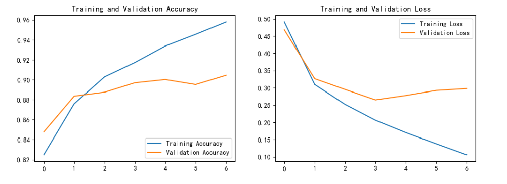
)Epoch 1/10 147/147 [==============================] - 1032s 7s/step - loss: 0.4909 - accuracy: 0.8249 - val_loss: 0.4680 - val_accuracy: 0.8478 Epoch 2/10 147/147 [==============================] - 1031s 7s/step - loss: 0.3099 - accuracy: 0.8759 - val_loss: 0.3266 - val_accuracy: 0.8836 Epoch 3/10 147/147 [==============================] - 1040s 7s/step - loss: 0.2522 - accuracy: 0.9029 - val_loss: 0.2955 - val_accuracy: 0.8876 Epoch 4/10 147/147 [==============================] - 1048s 7s/step - loss: 0.2063 - accuracy: 0.9173 - val_loss: 0.2651 - val_accuracy: 0.8970 Epoch 5/10 147/147 [==============================] - 1048s 7s/step - loss: 0.1705 - accuracy: 0.9338 - val_loss: 0.2778 - val_accuracy: 0.9002 Epoch 6/10 147/147 [==============================] - 1026s 7s/step - loss: 0.1379 - accuracy: 0.9455 - val_loss: 0.2927 - val_accuracy: 0.8953 Epoch 7/10 147/147 [==============================] - ETA: 0s - loss: 0.1062 - accuracy: 0.9579Restoring model weights from the end of the best epoch: 4. 147/147 [==============================] - 1019s 7s/step - loss: 0.1062 - accuracy: 0.9579 - val_loss: 0.2981 - val_accuracy: 0.9045 Epoch 7: early stopping
# 获取实际训练轮数
actual_epochs = len(history.history['accuracy'])

acc = history.history['accuracy']
val_acc = history.history['val_accuracy']

loss = history.history['loss']
val_loss = history.history['val_loss']

epochs_range = range(actual_epochs)

plt.figure(figsize=(12, 4))

# 绘制准确率
plt.subplot(1, 2, 1)
plt.plot(epochs_range, acc, label='Training Accuracy')
plt.plot(epochs_range, val_acc, label='Validation Accuracy')
plt.legend(loc='lower right')
plt.title('Training and Validation Accuracy')

# 绘制损失
plt.subplot(1, 2, 2)
plt.plot(epochs_range, loss, label='Training Loss')
plt.plot(epochs_range, val_loss, label='Validation Loss')
plt.legend(loc='upper right')
plt.title('Training and Validation Loss')
plt.savefig('准确率.png')
plt.show()