网络服务商网站网页制作作业源代码
基于R 4.4.2版本演示
一、写在前面
上一期我们使用了R语言构建了随机森林,并尝试进行SHAP,然后被打脸了。好在偶然发现还有一个封装好的SHAPforxgboost包,全村的希望。
借助GPT就在尝试一下吧。
二、R代码实现Xgboost分类
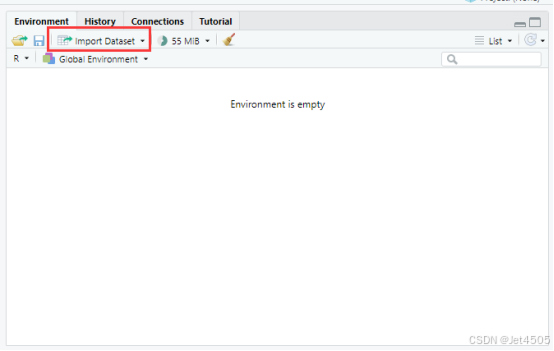
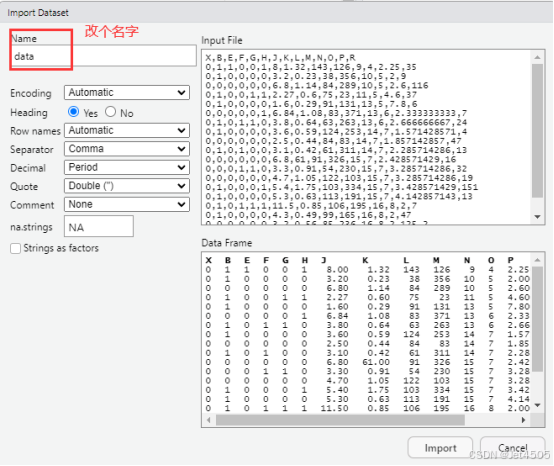
(1)导入数据
我习惯用RStudio自带的导入功能:

(2)建立Xgboost模型(默认参数)
# Load necessary libraries
library(caret)
library(pROC)
library(ggplot2)
library(xgboost)# Assume 'data' is your dataframe containing the data
# Set seed to ensure reproducibility
set.seed(123)# Split data into training and validation sets (80% training, 20% validation)
trainIndex <- createDataPartition(data$X, p = 0.8, list = FALSE)
trainData <- data[trainIndex, ]
validData <- data[-trainIndex, ]# Prepare matrices for XGBoost
dtrain <- xgb.DMatrix(data = as.matrix(trainData[, -which(names(trainData) == "X")]), label = trainData$X)
dvalid <- xgb.DMatrix(data = as.matrix(validData[, -which(names(validData) == "X")]), label = validData$X)# Define parameters for XGBoost
params <- list(booster = "gbtree", objective = "binary:logistic", eta = 0.1, gamma = 0, max_depth = 6, min_child_weight = 1, subsample = 0.8, colsample_bytree = 0.8)# Train the XGBoost model
model <- xgb.train(params = params, data = dtrain, nrounds = 100, watchlist = list(eval = dtrain), verbose = 1)# Predict on the training and validation sets
trainPredict <- predict(model, dtrain)
validPredict <- predict(model, dvalid)# Convert predictions to binary using 0.5 as threshold
#trainPredict <- ifelse(trainPredict > 0.5, 1, 0)
#validPredict <- ifelse(validPredict > 0.5, 1, 0)# Calculate ROC curves and AUC values
#trainRoc <- roc(response = trainData$X, predictor = as.numeric(trainPredict))
#validRoc <- roc(response = validData$X, predictor = as.numeric(validPredict))
trainRoc <- roc(response = as.numeric(trainData$X) - 1, predictor = trainPredict)
validRoc <- roc(response = as.numeric(validData$X) - 1, predictor = validPredict)# Plot ROC curves with AUC values
ggplot(data = data.frame(fpr = trainRoc$specificities, tpr = trainRoc$sensitivities), aes(x = 1 - fpr, y = tpr)) +geom_line(color = "blue") +geom_area(alpha = 0.2, fill = "blue") +geom_abline(slope = 1, intercept = 0, linetype = "dashed", color = "black") +ggtitle("Training ROC Curve") +xlab("False Positive Rate") +ylab("True Positive Rate") +annotate("text", x = 0.5, y = 0.1, label = paste("Training AUC =", round(auc(trainRoc), 2)), hjust = 0.5, color = "blue")ggplot(data = data.frame(fpr = validRoc$specificities, tpr = validRoc$sensitivities), aes(x = 1 - fpr, y = tpr)) +geom_line(color = "red") +geom_area(alpha = 0.2, fill = "red") +geom_abline(slope = 1, intercept = 0, linetype = "dashed", color = "black") +ggtitle("Validation ROC Curve") +xlab("False Positive Rate") +ylab("True Positive Rate") +annotate("text", x = 0.5, y = 0.2, label = paste("Validation AUC =", round(auc(validRoc), 2)), hjust = 0.5, color = "red")# Calculate confusion matrices based on 0.5 cutoff for probability
confMatTrain <- table(trainData$X, trainPredict >= 0.5)
confMatValid <- table(validData$X, validPredict >= 0.5)# Function to plot confusion matrix using ggplot2
plot_confusion_matrix <- function(conf_mat, dataset_name) {conf_mat_df <- as.data.frame(as.table(conf_mat))colnames(conf_mat_df) <- c("Actual", "Predicted", "Freq")p <- ggplot(data = conf_mat_df, aes(x = Predicted, y = Actual, fill = Freq)) +geom_tile(color = "white") +geom_text(aes(label = Freq), vjust = 1.5, color = "black", size = 5) +scale_fill_gradient(low = "white", high = "steelblue") +labs(title = paste("Confusion Matrix -", dataset_name, "Set"), x = "Predicted Class", y = "Actual Class") +theme_minimal() +theme(axis.text.x = element_text(angle = 45, hjust = 1), plot.title = element_text(hjust = 0.5))print(p)
}# Now call the function to plot and display the confusion matrices
plot_confusion_matrix(confMatTrain, "Training")
plot_confusion_matrix(confMatValid, "Validation")# Extract values for calculations
a_train <- confMatTrain[1, 1]
b_train <- confMatTrain[1, 2]
c_train <- confMatTrain[2, 1]
d_train <- confMatTrain[2, 2]a_valid <- confMatValid[1, 1]
b_valid <- confMatValid[1, 2]
c_valid <- confMatValid[2, 1]
d_valid <- confMatValid[2, 2]# Training Set Metrics
acc_train <- (a_train + d_train) / sum(confMatTrain)
error_rate_train <- 1 - acc_train
sen_train <- d_train / (d_train + c_train)
sep_train <- a_train / (a_train + b_train)
precision_train <- d_train / (b_train + d_train)
F1_train <- (2 * precision_train * sen_train) / (precision_train + sen_train)
MCC_train <- (d_train * a_train - b_train * c_train) / sqrt((d_train + b_train) * (d_train + c_train) * (a_train + b_train) * (a_train + c_train))
auc_train <- roc(response = trainData$X, predictor = trainPredict)$auc# Validation Set Metrics
acc_valid <- (a_valid + d_valid) / sum(confMatValid)
error_rate_valid <- 1 - acc_valid
sen_valid <- d_valid / (d_valid + c_valid)
sep_valid <- a_valid / (a_valid + b_valid)
precision_valid <- d_valid / (b_valid + d_valid)
F1_valid <- (2 * precision_valid * sen_valid) / (precision_valid + sen_valid)
MCC_valid <- (d_valid * a_valid - b_valid * c_valid) / sqrt((d_valid + b_valid) * (d_valid + c_valid) * (a_valid + b_valid) * (a_valid + c_valid))
auc_valid <- roc(response = validData$X, predictor = validPredict)$auc# Print Metrics
cat("Training Metrics\n")
cat("Accuracy:", acc_train, "\n")
cat("Error Rate:", error_rate_train, "\n")
cat("Sensitivity:", sen_train, "\n")
cat("Specificity:", sep_train, "\n")
cat("Precision:", precision_train, "\n")
cat("F1 Score:", F1_train, "\n")
cat("MCC:", MCC_train, "\n")
cat("AUC:", auc_train, "\n\n")cat("Validation Metrics\n")
cat("Accuracy:", acc_valid, "\n")
cat("Error Rate:", error_rate_valid, "\n")
cat("Sensitivity:", sen_valid, "\n")
cat("Specificity:", sep_valid, "\n")
cat("Precision:", precision_valid, "\n")
cat("F1 Score:", F1_valid, "\n")
cat("MCC:", MCC_valid, "\n")
cat("AUC:", auc_valid, "\n")
三、SHAPforxgboost包实现SHAP
直接上代码:
1. SHAP Summary Plot(摘要图)
# 加载必要库
library(tidyr)
library(ggplot2)# 计算SHAP值
shap_values <- predict(model, newdata = as.matrix(trainData[, -which(names(trainData) == "X")]), predcontrib = TRUE)# 将SHAP值转换为数据框
shap_values_df <- as.data.frame(shap_values)
colnames(shap_values_df) <- c(names(trainData[, -which(names(trainData) == "X")]), "BIAS")
shap_values_df <- shap_values_df[, -ncol(shap_values_df)]# 转为长格式
shap_long <- shap_values_df %>%pivot_longer(cols = everything(), names_to = "Feature", values_to = "SHAP_value")# 绘制SHAP Summary Plot(深蓝和深红)
ggplot(shap_long, aes(x = SHAP_value, y = Feature, color = SHAP_value)) +geom_jitter(width = 0.2, alpha = 0.6, size = 1) +scale_color_gradient2(low = "#08306B", mid = "white", high = "#A50F15", midpoint = 0) + theme_minimal() +labs(title = "SHAP Summary Plot",x = "SHAP Value (impact on model output)",y = "Feature",color = "SHAP Value") +theme(axis.text.y = element_text(size = 10),plot.title = element_text(hjust = 0.5))
输出:
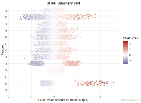
丑是丑了点,可以自行换颜色吧。
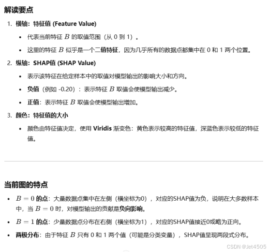
2. SHAP Dependence Plot(依赖图)
# 选择最重要的特征
top_feature <- colnames(shap_values_df)[1]
feature_values <- trainData[, top_feature]# 绘制依赖图
ggplot(data.frame(SHAP_value = shap_values_df[[top_feature]], Feature_value = feature_values),aes(x = Feature_value, y = SHAP_value, color = Feature_value)) +geom_point(alpha = 0.6) +scale_color_viridis(option = "plasma") +theme_minimal() +labs(title = paste("SHAP Dependence Plot -", top_feature),x = paste(top_feature, "Value"), y = "SHAP Value") +theme(legend.position = "none")
得出此图:
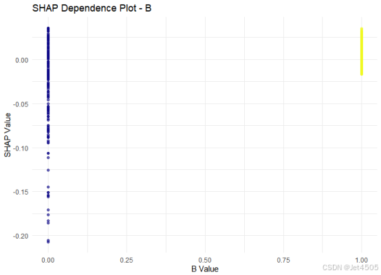
此图解读一下就是:
3. SHAP Force Plot(单样本解释)
# 选择第一个样本的SHAP值
shap_sample <- shap_values_df[1, ]
shap_sample_long <- data.frame(Feature = names(shap_sample), SHAP_value = as.numeric(shap_sample))# 绘制力图
ggplot(shap_sample_long, aes(x = reorder(Feature, SHAP_value), y = SHAP_value, fill = SHAP_value > 0)) +geom_bar(stat = "identity", color = "black") +scale_fill_manual(values = c("TRUE" = "#E41A1C", "FALSE" = "#377EB8")) + # 红蓝配色coord_flip() +theme_minimal() +labs(title = "SHAP Force Plot (Sample 1)", x = "Feature", y = "SHAP Value") +theme(legend.position = "none")
出图如下:
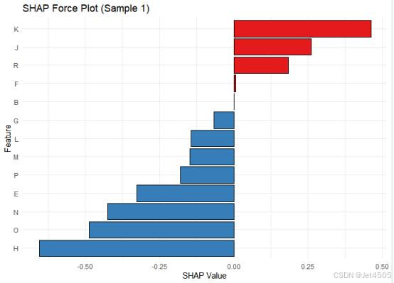
继续让GPT解读吧:
图中显示了:
第一个样本中各个特征的 SHAP 值,其中:
正向贡献特征(红色):特征 K、J 和 R 对模型输出产生了显著的正向贡献。
例如,特征 K 的 SHAP值接近 0.5,是当前样本中影响模型输出最大的正向特征。
负向贡献特征(蓝色):特征 H、O 和 N 等对模型输出产生了负向贡献。特征 H 的 SHAP值接近 -0.6,是当前样本中影响模型输出最大的负向特征。
零点:图中的竖直线表示模型的基准值(SHAP值为0),正向和负向贡献在此基础上抵消或加成,最终形成模型的输出预测值。
四、最后
老老实实用Python吧。
数据如下:
链接:https://pan.baidu.com/s/1rEf6JZyzA1ia5exoq5OF7g?pwd=x8xm
提取码:x8xm