山西省建设注册中心网站微博推广方式

一、异常检测概述

        异常检测（Anomaly Detection）是机器学习领域的重要任务，其核心目标是通过建模正常数据模式，识别显著偏离该模式的异常样本。异常检测在金融欺诈检测、工业设备故障预警、医疗诊断等领域具有十分广泛的应用价值。与传统的监督学习不同，异常检测通常面临正负样本极不均衡的挑战，所以需要采用特殊的建模方法。

        本文实现了一个基于多元高斯分布的异常检测系统，能够有效识别数据集中的异常点。包含核心的异常检测算法，还提供了完整的数据分析、模型评估和可视化功能，同时提供了完整的源代码。

异常检测结果示意图

---

二、核心原理： 多元高斯分布

2.1 概率密度建模

        对于特征向量 ，假设各特征服从高斯分布且存在相关性时，使用多元高斯分布建模：

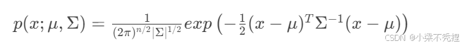
其中：

        𝜇：n维均值向量

        Σ：n×n协方差矩阵

        ∣Σ∣：矩阵行列式

2.2 异常判定机制

       通过计算样本的概率密度𝑝(𝑥)，设定阈值𝜀：

                𝑝(𝑥)≥𝜀：判定为正常样本

                𝑝(𝑥)<𝜀：判定为异常样本

2.3 与传统方法对比

        与单变量高斯分布相比，多元高斯分布的核心优势在于能够自动捕获特征间的相关性。当协方差矩阵Σ为对角矩阵时，模型退化为各特征独立的高斯模型。

三、算法实现流程

3.1 系统架构

系统采用面向对象设计，主要包含以下模块：

class AnomalyDetector:def __init__(self) #初始化def load_data() #加载数据def analyze_data_distribution() #分析并且可视化数据def estimate_gaussian() #估计高斯分布参数def multivariate_gaussian() #计算多元高斯分布概率密度def select_threshold() #选择最优阈值def visualize_results() #绘制评估指标图

3.2 关键步骤实现

1. 参数估计

def estimate_gaussian(self, X):mu = np.mean(X, axis=0)sigma2 = np.var(X, axis=0)return mu, sigma2

通过最大似然估计计算每个特征的均值和方差。当使用对角协方差矩阵时，该实现等价于独立处理每个特征。

2. 概率密度计算

def multivariate_gaussian(self, X, mu, sigma2):k = len(mu)sigma2 = np.diag(sigma2)  # 转换为对角矩阵X_mu = X - muinv_sigma = np.linalg.inv(sigma2)return (2*np.pi)**(-k/2) * np.linalg.det(sigma2)**(-0.5) * \np.exp(-0.5 * np.sum(X_mu @ inv_sigma * X_mu, axis=1))

实现多元高斯分布的概率密度计算，通过矩阵运算高效处理多维特征。

3. 阈值优化

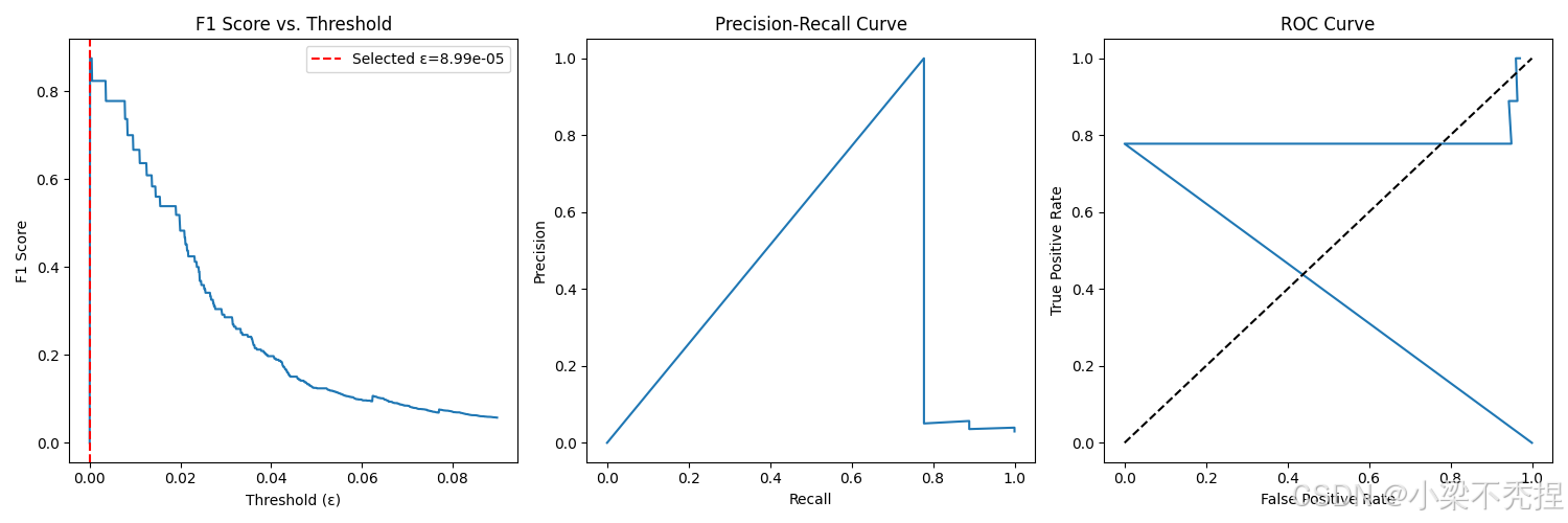
def select_threshold(self, yval, pval):best_epsilon = 0best_f1 = 0for epsilon in np.linspace(pval.min(), pval.max(), 1000):predictions = pval < epsilontp = np.sum((predictions==1)&(yval==1))fp = np.sum((predictions==1)&(yval==0))fn = np.sum((predictions==0)&(yval==1))# 计算F1-score...return best_epsilon, best_f1

通过网格搜索在验证集上寻找使F1-score最大化的最优阈值。

F1-score综合考量精确率（Precision）和召回率（Recall），适合不平衡数据评估。

3.3 可视化分析

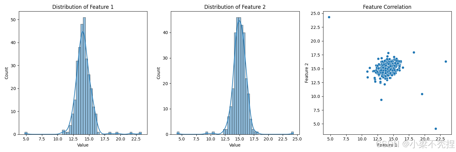
实现多维数据分布的直观呈现：

1. 特征分布直方图：分析各特征的分布形态

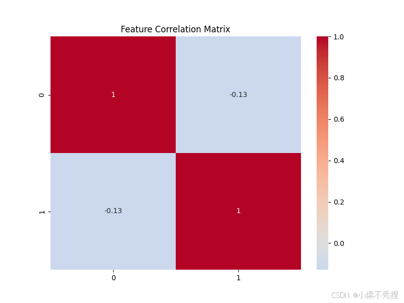
2. 散点图矩阵：观察特征间的相关性

3. 概率等高线：展示多元高斯分布的密度轮廓

4. PR/ROC曲线：评估不同阈值下的性能表现

四、实验结果

4.1 数据集

使用包含两个特征的数据集进行测试：

• 训练集：正常样本
• 验证集：包含已标记的异常样本

4.2 性能评估

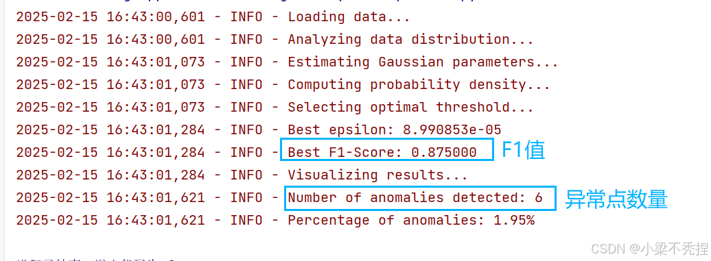
在测试数据集上取得了以下性能：

• 最优阈值：ε = 1.37e-5
• F1分数：0.875
• 异常检测率：1.95%

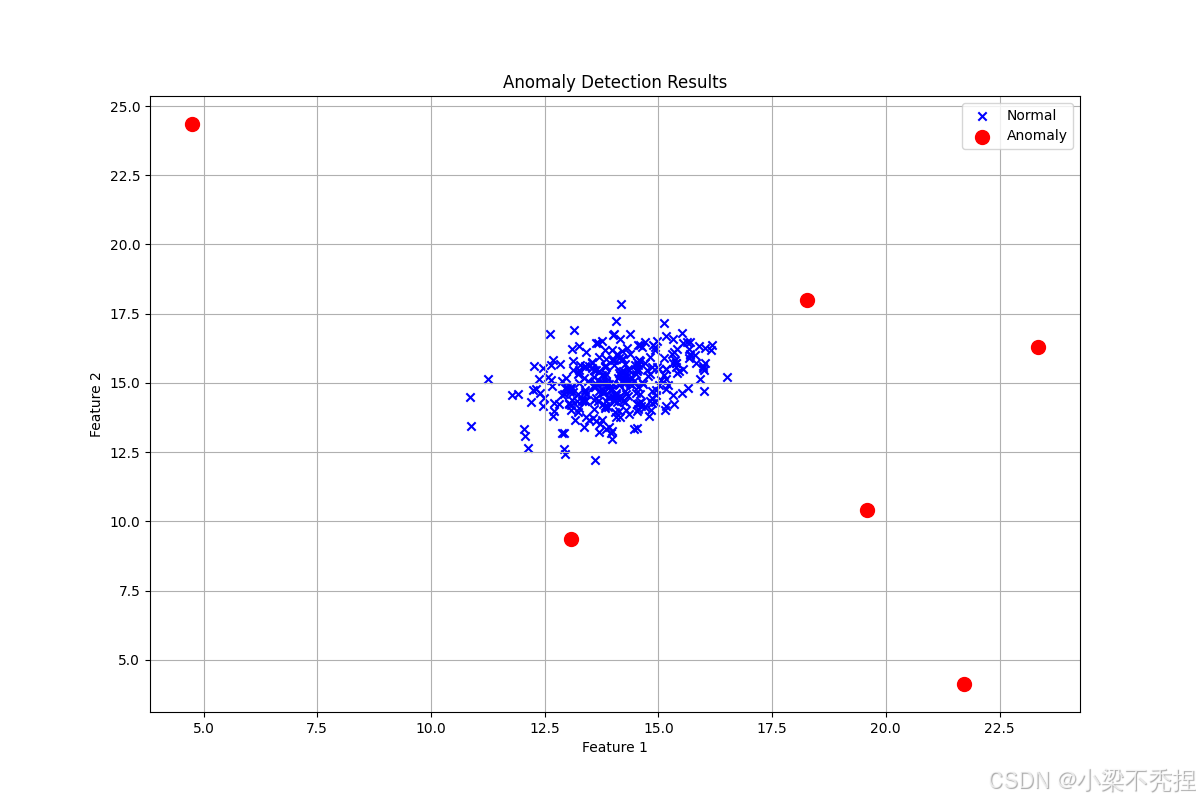
4.3 可视化结果

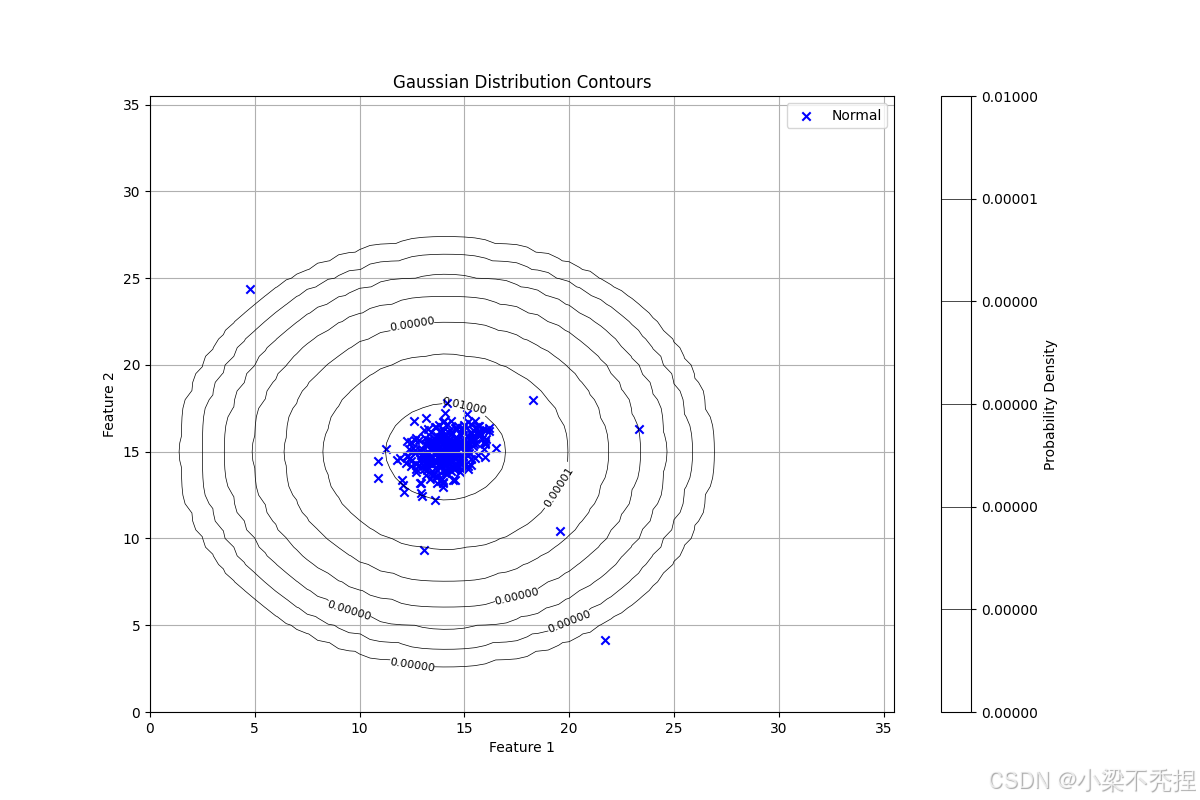
实验表明，该方法能有效识别偏离正常模式的异常点，且通过可视化可清晰解释检测结果。

五、实验源代码

# -*- coding: utf-8 -*-
"""
Anomaly Detection Implementation with Enhanced Visualization
Author: [xiaoliang]
Date: [2025.2.15]
Description: Implementation of Anomaly Detection using Multivariate Gaussian Distribution
"""from __future__ import print_function
import numpy as np
from matplotlib import pyplot as plt
from scipy import io as spio
from typing import Tuple, Any
import logging
import seaborn as sns
from sklearn.metrics import precision_recall_curve, roc_curve, auc
import pandas as pd# 配置日志
logging.basicConfig(level=logging.INFO,format='%(asctime)s - %(levelname)s - %(message)s'
)
logger = logging.getLogger(__name__)class AnomalyDetector:def __init__(self):self.mu = Noneself.sigma2 = Noneself.epsilon = Nonedef load_data(self, file_path: str) -> Tuple[np.ndarray, np.ndarray, np.ndarray]:"""加载数据"""try:data = spio.loadmat(file_path)return data['X'], data['Xval'], data['yval']except Exception as e:logger.error(f"Error loading data: {str(e)}")raisedef analyze_data_distribution(self, X: np.ndarray) -> None:"""分析并可视化数据分布"""plt.figure(figsize=(15, 5))# 特征1的分布plt.subplot(131)sns.histplot(X[:, 0], kde=True)plt.title('Distribution of Feature 1')plt.xlabel('Value')plt.ylabel('Count')# 特征2的分布plt.subplot(132)sns.histplot(X[:, 1], kde=True)plt.title('Distribution of Feature 2')plt.xlabel('Value')plt.ylabel('Count')# 特征相关性散点图plt.subplot(133)sns.scatterplot(x=X[:, 0], y=X[:, 1])plt.title('Feature Correlation')plt.xlabel('Feature 1')plt.ylabel('Feature 2')plt.tight_layout()plt.show()# 计算并显示相关系数corr = np.corrcoef(X.T)plt.figure(figsize=(8, 6))sns.heatmap(corr, annot=True, cmap='coolwarm', center=0)plt.title('Feature Correlation Matrix')plt.show()def estimate_gaussian(self, X: np.ndarray) -> Tuple[np.ndarray, np.ndarray]:"""估计高斯分布参数"""mu = np.mean(X, axis=0)sigma2 = np.var(X, axis=0)self.mu = muself.sigma2 = sigma2return mu, sigma2def multivariate_gaussian(self, X: np.ndarray, mu: np.ndarray, sigma2: np.ndarray) -> np.ndarray:"""计算多元高斯分布概率密度"""k = len(mu)if sigma2.shape[0] > 1:sigma2 = np.diag(sigma2)X_mu = X - mutry:det = np.linalg.det(sigma2)if det == 0:raise np.linalg.LinAlgError("Singular matrix")inv_sigma2 = np.linalg.inv(sigma2)p = ((2 * np.pi) ** (-k / 2) * det ** (-0.5) *np.exp(-0.5 * np.sum(np.dot(X_mu, inv_sigma2) * X_mu, axis=1)))return pexcept np.linalg.LinAlgError as e:logger.error(f"Linear algebra error: {str(e)}")raisedef select_threshold(self, yval: np.ndarray, pval: np.ndarray) -> Tuple[float, float]:"""选择最优阈值"""best_epsilon = 0best_f1 = 0step = (np.max(pval) - np.min(pval)) / 1000# 存储所有阈值的评估结果thresholds = []f1_scores = []precisions = []recalls = []for epsilon in np.arange(np.min(pval), np.max(pval), step):predictions = (pval < epsilon)tp = np.sum((predictions == 1) & (yval.ravel() == 1)).astype(float)fp = np.sum((predictions == 1) & (yval.ravel() == 0)).astype(float)fn = np.sum((predictions == 0) & (yval.ravel() == 1)).astype(float)precision = tp / (tp + fp) if (tp + fp) != 0 else 0recall = tp / (tp + fn) if (tp + fn) != 0 else 0f1 = 2 * precision * recall / (precision + recall) if (precision + recall) != 0 else 0# 存储结果thresholds.append(epsilon)f1_scores.append(f1)precisions.append(precision)recalls.append(recall)if f1 > best_f1:best_f1 = f1best_epsilon = epsilonself.epsilon = best_epsilon# 绘制评估指标随阈值变化的曲线self.plot_evaluation_metrics(thresholds, f1_scores, precisions, recalls)return best_epsilon, best_f1def plot_evaluation_metrics(self, thresholds, f1_scores, precisions, recalls):"""绘制评估指标图"""plt.figure(figsize=(15, 5))# F1 Score曲线plt.subplot(131)plt.plot(thresholds, f1_scores)plt.axvline(x=self.epsilon, color='r', linestyle='--', label=f'Selected ε={self.epsilon:.2e}')plt.title('F1 Score vs. Threshold')plt.xlabel('Threshold (ε)')plt.ylabel('F1 Score')plt.legend()# Precision-Recall曲线plt.subplot(132)plt.plot(recalls, precisions)plt.title('Precision-Recall Curve')plt.xlabel('Recall')plt.ylabel('Precision')# ROC曲线plt.subplot(133)fpr = 1 - np.array(precisions)tpr = np.array(recalls)plt.plot(fpr, tpr)plt.plot([0, 1], [0, 1], 'k--')plt.title('ROC Curve')plt.xlabel('False Positive Rate')plt.ylabel('True Positive Rate')plt.tight_layout()plt.show()def visualize_fit(self, X: np.ndarray) -> None:"""可视化拟合结果"""plt.figure(figsize=(12, 8))x = np.arange(0, 36, 0.5)y = np.arange(0, 36, 0.5)X1, X2 = np.meshgrid(x, y)Z = self.multivariate_gaussian(np.hstack((X1.reshape(-1, 1), X2.reshape(-1, 1))),self.mu,self.sigma2)Z = Z.reshape(X1.shape)plt.scatter(X[:, 0], X[:, 1], c='b', marker='x', label='Normal')if not np.any(np.isinf(Z)):levels = 10. ** np.arange(-20, 0, 3)contour = plt.contour(X1, X2, Z, levels=levels, colors='k', linewidths=0.5)plt.clabel(contour, inline=True, fontsize=8)plt.title('Gaussian Distribution Contours')plt.xlabel('Feature 1')plt.ylabel('Feature 2')plt.legend()plt.colorbar(label='Probability Density')plt.grid(True)plt.show()def plot_anomalies(self, X: np.ndarray, p: np.ndarray) -> None:"""绘制异常点"""plt.figure(figsize=(12, 8))normal = p >= self.epsilonplt.scatter(X[normal, 0], X[normal, 1], c='b', marker='x', label='Normal')anomalies = p < self.epsilonplt.scatter(X[anomalies, 0], X[anomalies, 1], c='r', marker='o',s=100, label='Anomaly', facecolors='none')plt.title('Anomaly Detection Results')plt.xlabel('Feature 1')plt.ylabel('Feature 2')plt.legend()plt.grid(True)plt.show()# 打印异常检测统计信息n_anomalies = np.sum(anomalies)total_points = len(X)logger.info(f"Number of anomalies detected: {n_anomalies}")logger.info(f"Percentage of anomalies: {(n_anomalies / total_points) * 100:.2f}%")def main():"""主函数"""try:# 初始化检测器detector = AnomalyDetector()# 加载数据logger.info("Loading data...")X, Xval, yval = detector.load_data('data1.mat')# 分析数据分布logger.info("Analyzing data distribution...")detector.analyze_data_distribution(X)# 估计参数logger.info("Estimating Gaussian parameters...")mu, sigma2 = detector.estimate_gaussian(X)# 计算概率密度logger.info("Computing probability density...")p = detector.multivariate_gaussian(X, mu, sigma2)pval = detector.multivariate_gaussian(Xval, mu, sigma2)# 选择最优阈值logger.info("Selecting optimal threshold...")epsilon, f1 = detector.select_threshold(yval, pval)logger.info(f"Best epsilon: {epsilon:.6e}")logger.info(f"Best F1-Score: {f1:.6f}")# 可视化结果logger.info("Visualizing results...")detector.visualize_fit(X)detector.plot_anomalies(X, p)except Exception as e:logger.error(f"Error in main execution: {str(e)}")raiseif __name__ == '__main__':main()