当前位置：首页 > news >正文

快速上手大模型：机器学习4（特征缩放、学习率选择）

news 2025/10/20 20:04:53

1 特征缩放

1.1 引子

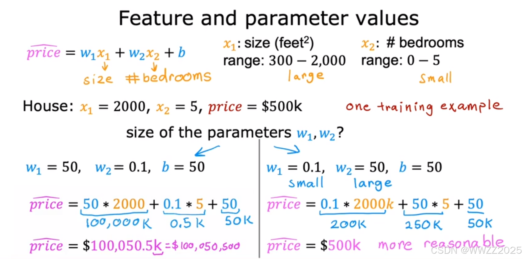
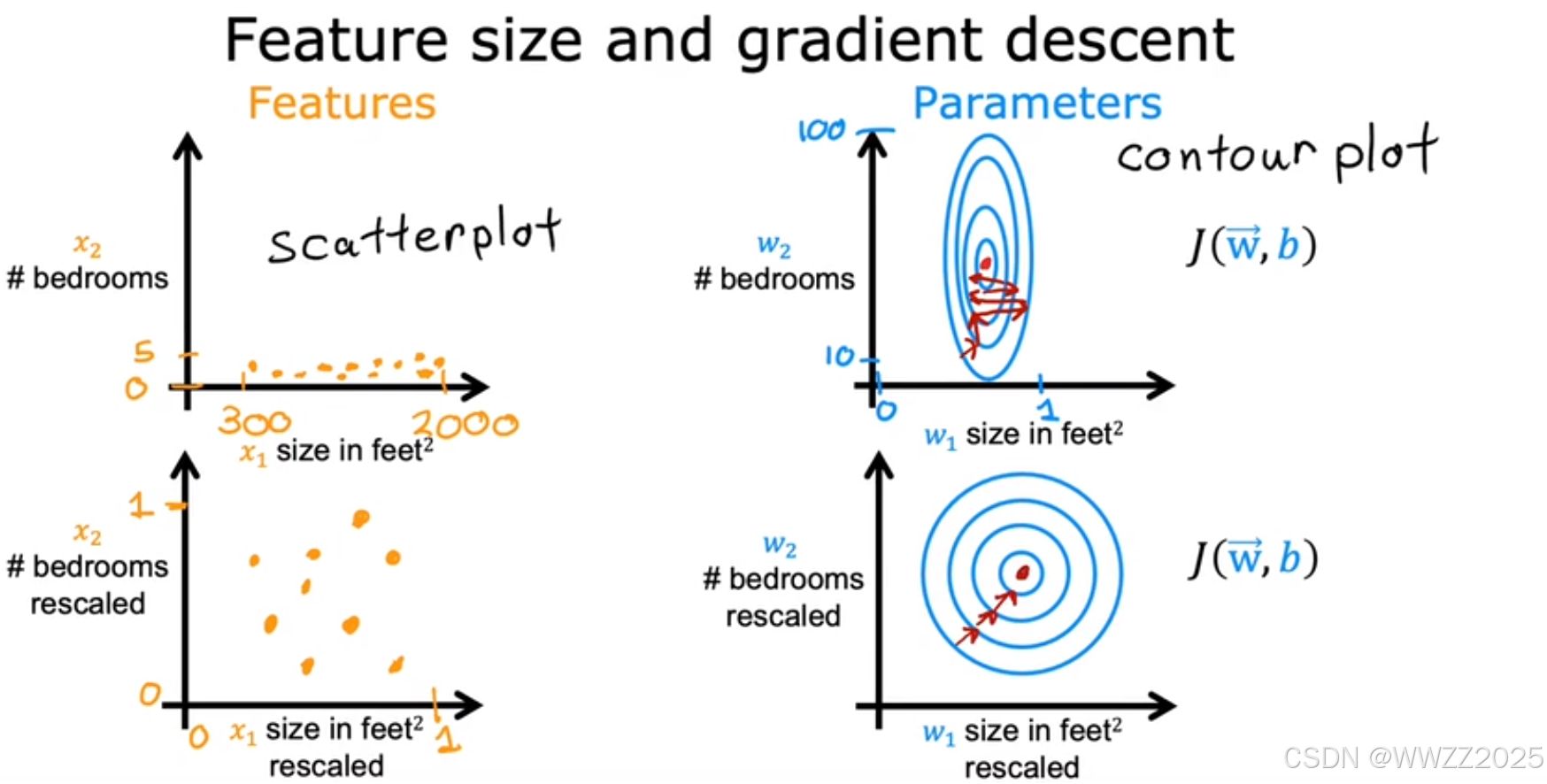
结论：通过缩放w1*x1、w2*x2使其数值差接近，使用转换后的数据运行梯度下降算法，等高线类似于圆，梯度下降可以找到一条更直接的路径到达全局最小值。

1.2 缩放方法

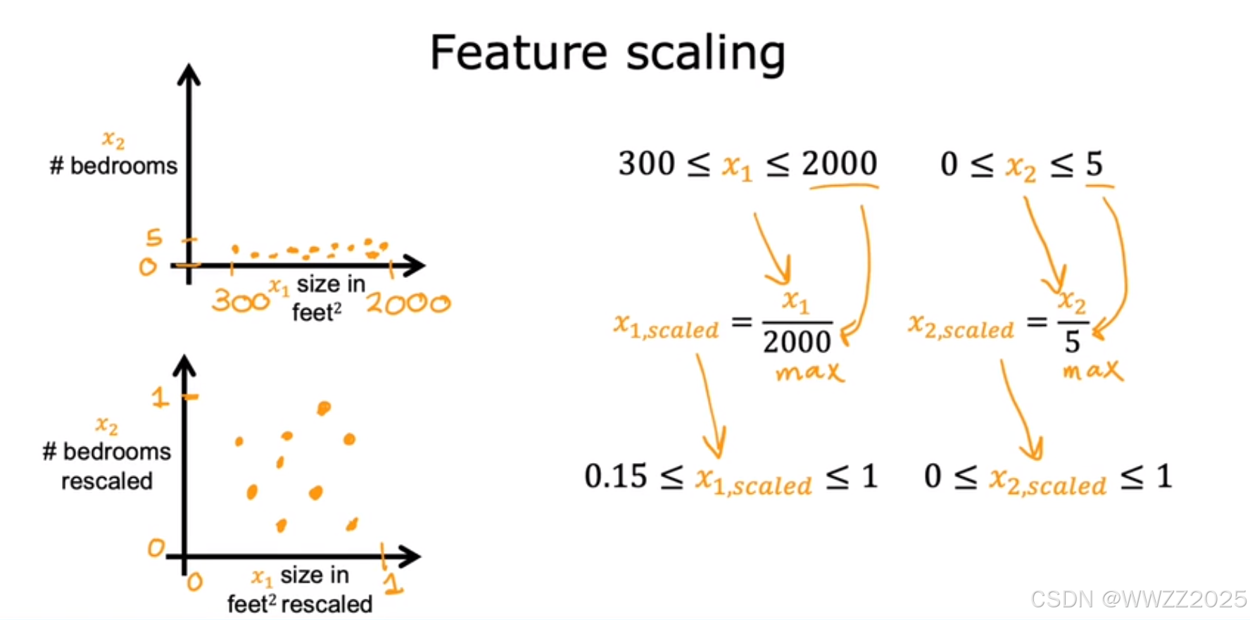
1.2.1 除以最大值法

除以区间最大值，使缩放后的点落在一个近圆上。

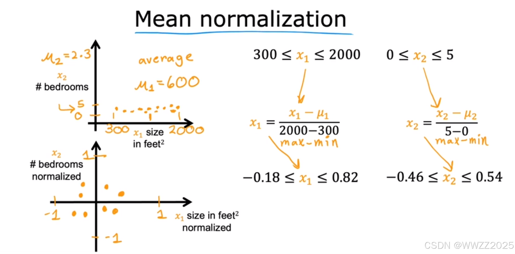
1.2.2 均值归一化(Mean normalization)

缩放后使x1、x2在-1～1之间分布。 $\mu _{1}$ 、 $\mu _{2}$ 分别是x1、x2在训练集上的均值，然后用每个x1、x2算放缩后的值，找出放缩后的范围。

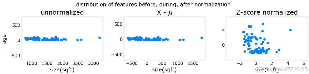
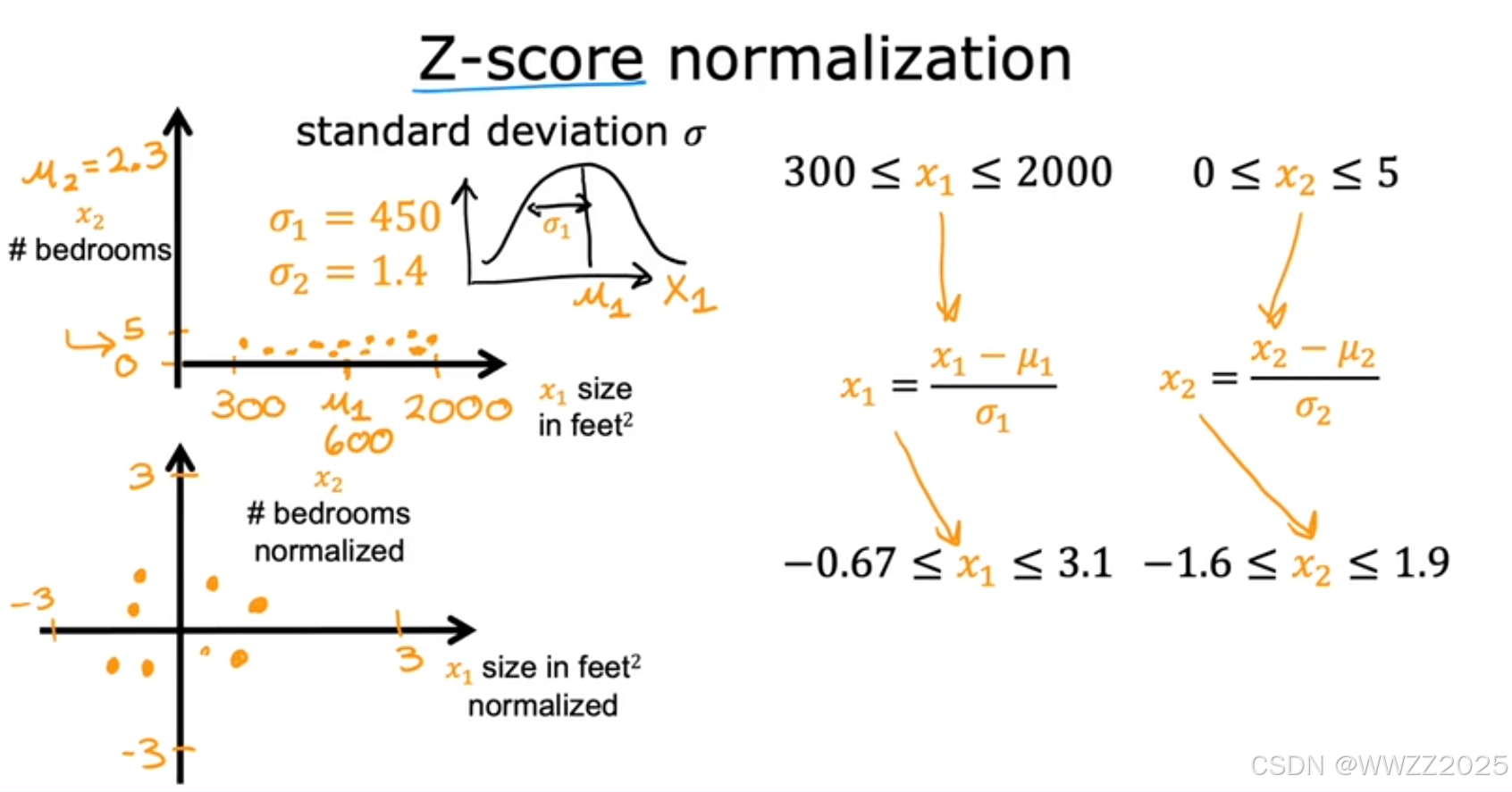
1.2.3 Z-score归一化(Z-score normalization)

归一化公式： $x_{1}=\frac{x_{1}-\mu _{1}}{\sigma _{1}}$ ， $x_{2}=\frac{x_{2}-\mu _{2}}{\sigma _{2}}$

其中， $\mu _{1},\mu _{2}$ 分别是x1、x2在训练集上的均值； $\sigma _{1},\sigma _{2}$ 是标准差( $\sigma =\sqrt{\frac{\sum_{i=1}^{N}(x_{i}-\mu )^{2}}{N}}$ )

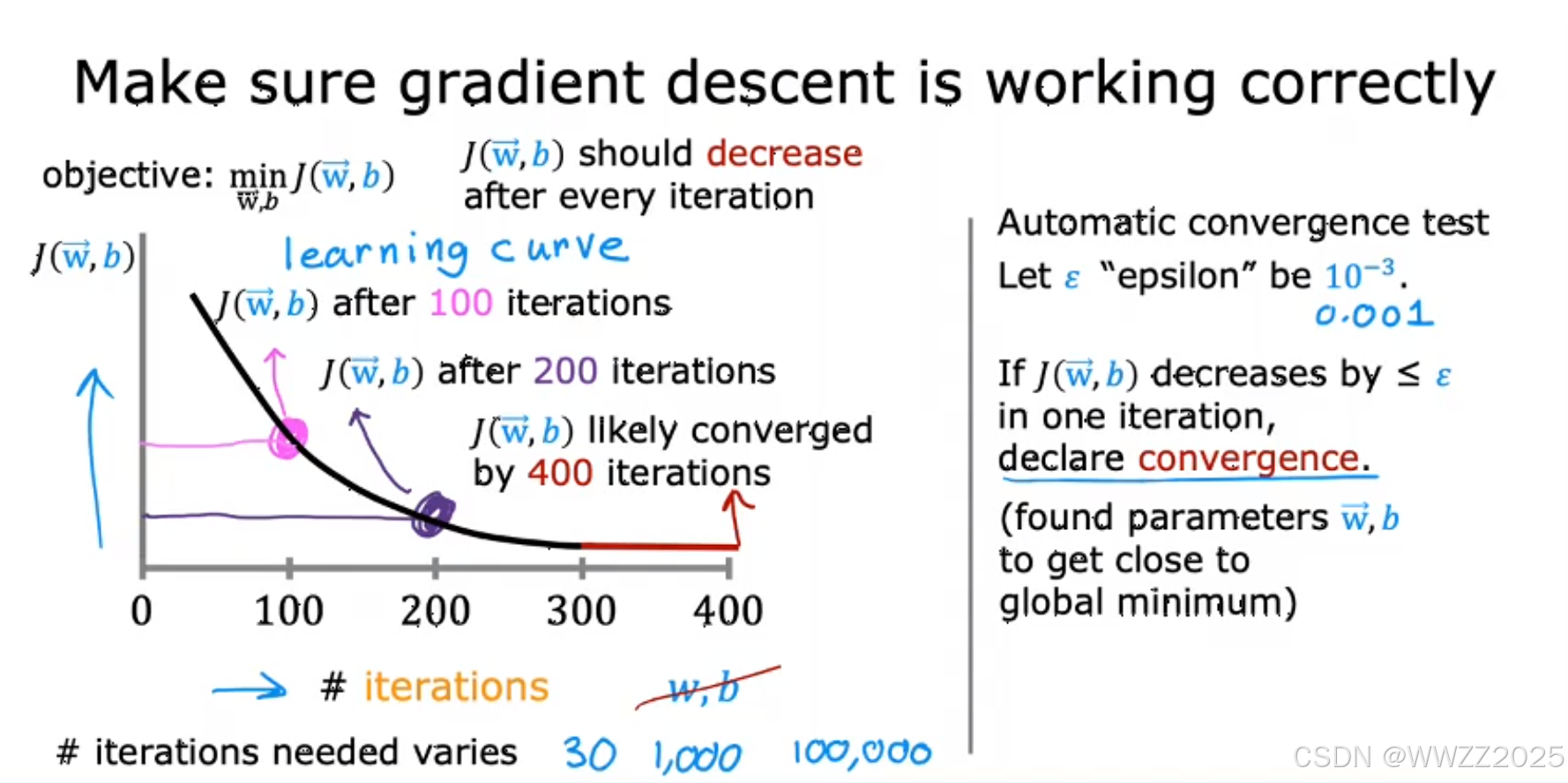
2 梯度下降收敛判断

法1：

观察左侧曲线图，迭代至一定次数后基本不再下降，此时即认为收敛。

法2：

自动收敛测试，当J< $\varepsilon$ 时认为收敛， $\varepsilon$ 为设定值，实际使用时不好找，常用法1。

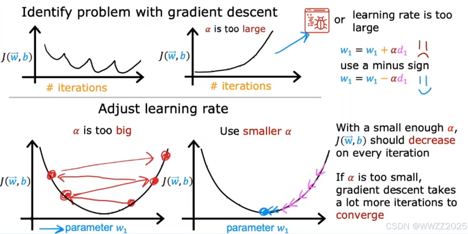
3 学习率选择（步长）

3.1 理论

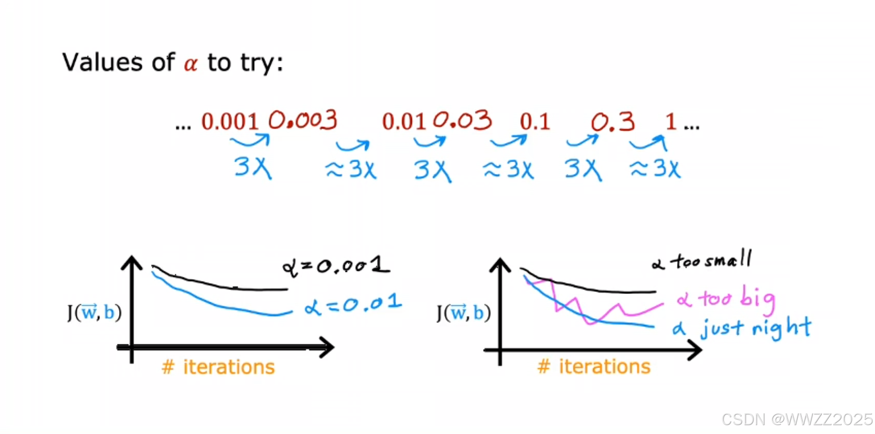
结论：学习率不宜过大或过小，过大出现发散，过小则需要通过更多的迭代次数才能达到收敛。

学习率选择：

从0.001开始，0.01、0.1、1进行选择，十倍频程，直至找到蓝色曲线。

3.2 代码实现

3.2.1 代价函数及参数运算

#set alpha to 9.9e-7
_, _, hist = run_gradient_descent(X_train, y_train, 10, alpha = 9.9e-7)

输出：

Iteration Cost          w0       w1       w2       w3       b       djdw0    djdw1    djdw2    djdw3    djdb  
---------------------|--------|--------|--------|--------|--------|--------|--------|--------|--------|--------|0 9.55884e+04  5.5e-01  1.0e-03  5.1e-04  1.2e-02  3.6e-04 -5.5e+05 -1.0e+03 -5.2e+02 -1.2e+04 -3.6e+021 1.28213e+05 -8.8e-02 -1.7e-04 -1.0e-04 -3.4e-03 -4.8e-05  6.4e+05  1.2e+03  6.2e+02  1.6e+04  4.1e+022 1.72159e+05  6.5e-01  1.2e-03  5.9e-04  1.3e-02  4.3e-04 -7.4e+05 -1.4e+03 -7.0e+02 -1.7e+04 -4.9e+023 2.31358e+05 -2.1e-01 -4.0e-04 -2.3e-04 -7.5e-03 -1.2e-04  8.6e+05  1.6e+03  8.3e+02  2.1e+04  5.6e+024 3.11100e+05  7.9e-01  1.4e-03  7.1e-04  1.5e-02  5.3e-04 -1.0e+06 -1.8e+03 -9.5e+02 -2.3e+04 -6.6e+025 4.18517e+05 -3.7e-01 -7.1e-04 -4.0e-04 -1.3e-02 -2.1e-04  1.2e+06  2.1e+03  1.1e+03  2.8e+04  7.5e+026 5.63212e+05  9.7e-01  1.7e-03  8.7e-04  1.8e-02  6.6e-04 -1.3e+06 -2.5e+03 -1.3e+03 -3.1e+04 -8.8e+027 7.58122e+05 -5.8e-01 -1.1e-03 -6.2e-04 -1.9e-02 -3.4e-04  1.6e+06  2.9e+03  1.5e+03  3.8e+04  1.0e+038 1.02068e+06  1.2e+00  2.2e-03  1.1e-03  2.3e-02  8.3e-04 -1.8e+06 -3.3e+03 -1.7e+03 -4.2e+04 -1.2e+039 1.37435e+06 -8.7e-01 -1.7e-03 -9.1e-04 -2.7e-02 -5.2e-04  2.1e+06  3.9e+03  2.0e+03  5.1e+04  1.4e+03
w,b found by gradient descent: w: [-0.87 -0.   -0.   -0.03], b: -0.00

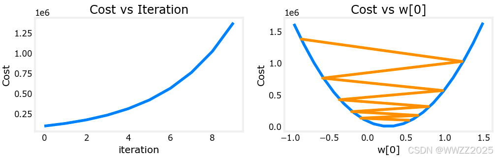
3.2.2 图像绘制

plot_cost_i_w(X_train, y_train, hist)

输出：

3.2.3 Z-score归一化

def zscore_normalize_features(X):"""computes  X, zcore normalized by columnArgs:X (ndarray): Shape (m,n) input data, m examples, n featuresReturns:X_norm (ndarray): Shape (m,n)  input normalized by columnmu (ndarray):     Shape (n,)   mean of each featuresigma (ndarray):  Shape (n,)   standard deviation of each feature"""# find the mean of each column/featuremu     = np.mean(X, axis=0)                 # mu will have shape (n,)# find the standard deviation of each column/featuresigma  = np.std(X, axis=0)                  # sigma will have shape (n,)# element-wise, subtract mu for that column from each example, divide by std for that columnX_norm = (X - mu) / sigma      return (X_norm, mu, sigma)#check our work
#from sklearn.preprocessing import scale
#scale(X_orig, axis=0, with_mean=True, with_std=True, copy=True)mu     = np.mean(X_train,axis=0)   
sigma  = np.std(X_train,axis=0) 
X_mean = (X_train - mu)
X_norm = (X_train - mu)/sigma      fig,ax=plt.subplots(1, 3, figsize=(12, 3))
ax[0].scatter(X_train[:,0], X_train[:,3])
ax[0].set_xlabel(X_features[0]); ax[0].set_ylabel(X_features[3]);
ax[0].set_title("unnormalized")
ax[0].axis('equal')ax[1].scatter(X_mean[:,0], X_mean[:,3])
ax[1].set_xlabel(X_features[0]); ax[0].set_ylabel(X_features[3]);
ax[1].set_title(r"X - $\mu$")
ax[1].axis('equal')ax[2].scatter(X_norm[:,0], X_norm[:,3])
ax[2].set_xlabel(X_features[0]); ax[0].set_ylabel(X_features[3]);
ax[2].set_title(r"Z-score normalized")
ax[2].axis('equal')
plt.tight_layout(rect=[0, 0.03, 1, 0.95])
fig.suptitle("distribution of features before, during, after normalization")
plt.show()

输出：