使用扩散模型DDPM生成Sine正弦曲线的案例（使用Classifier-free guidance）

简介

生成式扩散模型已经成为生成式人工智能的基础。对于工程上常见的数据生成任务（曲线、向量并非图像），并不需要用到相对复杂的U-Net和注意力机制，只需要普通的全连接神经网络即可搭建扩散模型。

本文则提供一个简易的代码，仅使用全连接神经网络实现Sine正弦曲线的生成任务。所搭建的扩散模型需要输入振幅、频率和相位三个条件（Condition），可从高斯噪声出发，一步一步去噪，并使用Classifier-free guidance技术，得到近似符合条件的Sine函数。

本文的代码可以作为一个学习案例，读者可根据具体工程问题，将三个条件（Condition）扩充，实现其他数据生成任务。

方法

代码改编自
https://github.com/cloneofsimo/minDiffusion
and
https://github.com/TeaPearce/Conditional_Diffusion_MNIST
扩散模型理论源于
https://arxiv.org/abs/2006.11239
条件引导的理论源于
https://arxiv.org/abs/2207.12598

代码

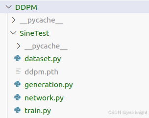
代码由dataset.py, generation.py, network.py, train.py四个文件构成，文件目录如下

dataset.py用于定义训练用的数据集，也就是随机生成的正弦曲线，曲线由数列表示。

from torch.utils.data import Dataset
import numpy as np

# 自定义数据集类
class SinWaveDataset(Dataset):
    def __init__(self, num_samples, sequence_length):
        self.num_samples = num_samples
        self.sequence_length = sequence_length
        self.data, self.labels = self.generate_data()

    def generate_data(self):
        data = []
        labels = []

        for _ in range(self.num_samples):
            t = np.linspace(0, 4*np.pi, self.sequence_length)  # 时间点
            freq = np.random.uniform(1.0, 10.0)  # 随机频率
            amplitude = np.random.uniform(0.5, 2.0)  # 随机振幅
            phase = np.random.uniform(0, 2 * np.pi)  # 随机相位
            x = amplitude * np.sin(freq * t + phase)  # 生成x数值
            condition=np.array([amplitude, freq, phase])
            data.append(x)  # 每个样本是 (sequence_length)
            labels.append(condition)  # 振幅、频率、相位作为标签

        data = np.array(data, dtype=np.float32)
        labels = np.array(labels, dtype=np.float32)
        return data, labels

    def __len__(self):
        return self.num_samples

    def __getitem__(self, idx):
        return self.data[idx], self.labels[idx]

network.py用于定义神经网络, FCNN是全连接神经网络，EmbedFC是全连接嵌入层，ddpm_schedules定义了扩散模型加噪规律，DDPM的forward用于预测噪声，DDPM的sample用于完成训练后的数据生成

import torch
import torch.nn as nn
import numpy as np

# GPU or CPU
device = torch.device(
    "cuda") if torch.cuda.is_available() else torch.device("cpu")


class FCNN(nn.Module):
    def __init__(self, hidden_sizes, x_size, time_embed_size, condition_size, condition_embed_size):
        super(FCNN, self).__init__()
        input_size = x_size + time_embed_size + condition_embed_size
        bypass_size = time_embed_size + condition_embed_size

        self.layers = nn.ModuleList()
        self.bn_layers = nn.ModuleList()

        # First layer
        self.layers.append(nn.Linear(input_size, hidden_sizes[0]))
        self.bn_layers.append(nn.BatchNorm1d(hidden_sizes[0]))

        # Hidden layers
        for i in range(1, len(hidden_sizes)):
            self.layers.append(
                nn.Linear(hidden_sizes[i - 1] + bypass_size, hidden_sizes[i]))
            self.bn_layers.append(nn.BatchNorm1d(hidden_sizes[i]))

        # Output layer
        self.layers.append(nn.Linear(hidden_sizes[-1] + bypass_size, x_size))

        self.leaky_relu = nn.LeakyReLU(0.01)
        self.dropout = nn.Dropout(0.05)

        self.time_embeding = EmbedFC(1, time_embed_size)
        self.condition_embeding = EmbedFC(condition_size, condition_embed_size)

    def forward(self, x, time, condition, context_mask):
        time_embed = self.time_embeding(time)
        condition_embed = self.condition_embeding(
            condition) * (1.0 - context_mask)
        for i, layer in enumerate(self.layers[:-1]):
            x = torch.cat((x, time_embed, condition_embed), 1)
            x = layer(x)
            x = self.leaky_relu(x)
            x = self.bn_layers[i](x)
            x = self.dropout(x)

        x = torch.cat((x, time_embed, condition_embed), 1)
        x = self.layers[-1](x)

        return x

# A fully connected neural network for embed
class EmbedFC(nn.Module):
    def __init__(self, input_dim, emb_dim):
        super(EmbedFC, self).__init__()
        self.input_dim = input_dim
        layers = [
            nn.Linear(input_dim, emb_dim)
        ]
        self.model = nn.Sequential(*layers)

    def forward(self, x):
        x = x.view(-1, self.input_dim)
        return self.model(x)

def ddpm_schedules(beta1, beta2, T):
    """
    Returns pre-computed schedules for DDPM sampling, training process.
    """
    assert beta1 < beta2 < 1.0, "beta1 and beta2 must be in (0, 1)"

    beta_t = (beta2 - beta1) * torch.arange(0, T +
                                            1, dtype=torch.float32) / T + beta1
    sqrt_beta_t = torch.sqrt(beta_t)
    alpha_t = 1 - beta_t
    log_alpha_t = torch.log(alpha_t)
    alphabar_t = torch.cumsum(log_alpha_t, dim=0).exp()

    sqrtab = torch.sqrt(alphabar_t)
    oneover_sqrta = 1 / torch.sqrt(alpha_t)

    sqrtmab = torch.sqrt(1 - alphabar_t)
    mab_over_sqrtmab_inv = (1 - alpha_t) / sqrtmab

    return {
        "alpha_t": alpha_t,  # \alpha_t
        "oneover_sqrta": oneover_sqrta,  # 1/\sqrt{\alpha_t}
        "sqrt_beta_t": sqrt_beta_t,  # \sqrt{\beta_t}
        "alphabar_t": alphabar_t,  # \bar{\alpha_t}
        "sqrtab": sqrtab,  # \sqrt{\bar{\alpha_t}}
        "sqrtmab": sqrtmab,  # \sqrt{1-\bar{\alpha_t}}
        # (1-\alpha_t)/\sqrt{1-\bar{\alpha_t}}
        "mab_over_sqrtmab": mab_over_sqrtmab_inv,
    }


class DDPM(nn.Module):
    def __init__(self, nn_model, betas, n_T, device, drop_prob=0.1):
        super(DDPM, self).__init__()
        self.nn_model = nn_model.to(device)
        num_params = sum(p.numel() for p in nn_model.parameters())
        print(f"Parameter number: {num_params*1e-6}M")
        # register_buffer allows accessing dictionary produced by ddpm_schedules
        # e.g. can access self.sqrtab later
        for k, v in ddpm_schedules(betas[0], betas[1], n_T).items():
            self.register_buffer(k, v)

        self.n_T = n_T
        self.device = device
        self.drop_prob = drop_prob
        self.loss_mse = nn.MSELoss()

    def forward(self, x, condition):
        """
        this method is used in training, so samples t and noise randomly
        """
        _ts = torch.randint(
            1, self.n_T+1, (x.shape[0],)).to(self.device)  # t ~ Uniform(0, n_T)
        noise = torch.randn_like(x)  # eps ~ N(0, 1)

        x_t = (
            self.sqrtab[_ts, None] * x
            + self.sqrtmab[_ts, None] * noise
        )  # This is the x_t, which is sqrt(alphabar) x_0 + sqrt(1-alphabar) * eps
        # We should predict the "error term" from this x_t. Loss is what we return.

        # dropout context with some probability
        context_mask = torch.bernoulli(
            torch.zeros_like(condition[:, 0:1])+self.drop_prob).to(self.device)

        # return MSE between added noise, and our predicted noise
        return self.loss_mse(noise, self.nn_model(x_t, _ts / self.n_T, condition, context_mask))

    def sample(self, n_sample, x_size, device, guide_w=0.0, condition=None):
        # we follow the guidance sampling scheme described in 'Classifier-Free Diffusion Guidance'
        # to make the fwd passes efficient, we concat two versions of the dataset,
        # one with context_mask=0 and the other context_mask=1
        # we then mix the outputs with the guidance scale, w
        # where w>0 means more guidance

        # x_T ~ N(0, 1), sample initial noise
        x_i = torch.randn(n_sample, x_size).to(device)
        condition = condition.unsqueeze(0).repeat(n_sample, 1).to(device)

        # don't drop context at test time
        context_mask = torch.zeros_like(condition[:, 0:1]).to(device)

        # double the batch
        condition = condition.repeat(2, 1)
        context_mask = context_mask.repeat(2, 1)
        context_mask[n_sample:] = 1.  # makes second half of batch context free
        x_i_store = []  # keep track of generated steps in case want to plot something
        for i in range(self.n_T, 0, -1):
            print(f'sampling timestep {i}\n')
            t_is = torch.tensor([i / self.n_T]).to(device)
            t_is = t_is.repeat(n_sample, 1)

            # double batch
            x_i = x_i.repeat(2, 1)
            t_is = t_is.repeat(2, 1)

            z = torch.randn(n_sample, x_size).to(device) if i > 1 else 0

            # split predictions and compute weighting
            eps = self.nn_model(x_i, t_is[:, 0], condition, context_mask)
            eps1 = eps[:n_sample]
            eps2 = eps[n_sample:]
            eps = (1.0+guide_w)*eps1 - guide_w*eps2
            x_i = x_i[:n_sample]

            x_i = (
                self.oneover_sqrta[i] * (x_i - eps * self.mab_over_sqrtmab[i])
                + self.sqrt_beta_t[i] * z
            )
            x_i_store.append(x_i.detach().cpu().numpy())
        x_i_store.reverse()
        x_i_store = np.array(x_i_store)
        x_i_store = torch.Tensor(x_i_store)
        return x_i, x_i_store

train.py用于训练神经网络

''' 
This script does conditional latent generation using a diffusion model

This code is modified from,
https://github.com/cloneofsimo/minDiffusion
and
https://github.com/TeaPearce/Conditional_Diffusion_MNIST

Diffusion model is based on DDPM,
https://arxiv.org/abs/2006.11239

The conditioning idea is taken from 'Classifier-Free Diffusion Guidance',
https://arxiv.org/abs/2207.12598

This technique also features in ImageGen 'Photorealistic Text-to-Image Diffusion Modelswith Deep Language Understanding',
https://arxiv.org/abs/2205.11487

'''
from tqdm import tqdm
import torch
from torch.utils.data import DataLoader
import matplotlib.pyplot as plt
import math
from network import DDPM,FCNN
from dataset import SinWaveDataset

def main():
    device = torch.device(
    "cuda") if torch.cuda.is_available() else torch.device("cpu")
    # hardcoding of the training parameters
    n_epoch = 2000
    batch_size = 512
    n_T = 1000
    lrate = 1e-3

    x_size=128
    time_embed_size=64
    condition_size=3
    condition_embed_size=64

    ddpm = DDPM(nn_model=FCNN(hidden_sizes=[4096,4096,4096,4096],
                              x_size=x_size,
                              time_embed_size=time_embed_size,
                              condition_size=condition_size,
                              condition_embed_size=condition_embed_size),
                              betas=(1e-4, 0.02),
                              n_T=n_T,
                              device=device,
                              drop_prob=0.05)
    ddpm.to(device)
    # Create dataset
    train_dataset = SinWaveDataset(5000, 128)
    train_dataloader = DataLoader(train_dataset, batch_size=batch_size, shuffle=True, num_workers=5)

    optim = torch.optim.Adam(ddpm.parameters(), lr=lrate)

    losses = []

    for ep in range(n_epoch):
        print(f'epoch {ep}')
        ddpm.train()

        # Linear lrate decay
        optim.param_groups[0]['lr'] = lrate*(1-ep/n_epoch)

        pbar = tqdm(train_dataloader)
        loss_ema = None
        for x, c in pbar:
            optim.zero_grad()
            x = x.to(device)
            c = c.to(device)

            loss = ddpm(x, c)
            
            loss.backward()
            if loss_ema is None:
                loss_ema = loss.item()
            else:
                loss_ema = 0.95 * loss_ema + 0.05 * loss.item()
            pbar.set_description(f"loss: {loss_ema:.4f}")
            optim.step()
            losses.append(math.log(loss_ema)/math.log(10))

        # Draw loss curve
        plt.clf()
        plt.plot(losses)
        plt.xlabel('Steps')
        plt.ylabel('Loss')
        plt.title('Training Loss Curve')
        plt.pause(0.001)

        torch.save(ddpm, "DDPM/SineTest/ddpm.pth")
        print('model saved model')



if __name__ == "__main__":
    main()

generation.py用于训练完成后生成数据

import numpy as np
import torch
import matplotlib.pyplot as plt

# GPU or CPU
device = torch.device(
    "cuda") if torch.cuda.is_available() else torch.device("cpu")

def generate_samples(n_sample, condition, guide_w):
    with torch.no_grad():
        # Load trained DDPM model
        ddpm = torch.load("DDPM/SineTest/ddpm.pth", map_location=device)
        ddpm.eval()
        x_gen, x_gen_store = ddpm.sample(n_sample=n_sample, 
                                         x_size=128, 
                                         device=device, 
                                         guide_w=guide_w, 
                                         condition=condition)
        return x_gen

if __name__ == "__main__":
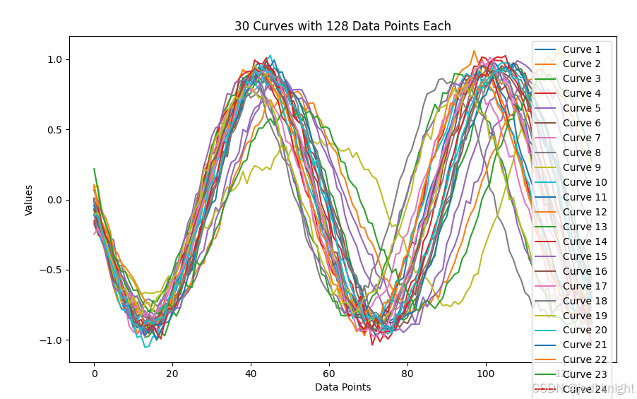
    condition=torch.tensor([1.5, 4.0, np.pi/2])#给定振幅、频率、相位
    # 生成样本
    out = generate_samples(n_sample = 30,
                         condition = condition,
                         guide_w = 1.0)
    out = out.cpu().numpy()
    
    # 创建一个图形
    plt.figure(figsize=(10, 6))

    # 遍历每一行数据并绘制曲线
    for i in range(out.shape[0]):
        plt.plot(out[i], label=f'Curve {i+1}')

    # 添加图例
    plt.legend()

    # 添加标题和轴标签
    plt.title('30 Curves with 128 Data Points Each')
    plt.xlabel('Data Points')
    plt.ylabel('Values')

    # 显示图形
    plt.show()
    

运行

运行train.py，训练完毕后可以得到ddpm.pth文件

运行generation.py，可以根据条件生成30组曲线，并绘制于窗口

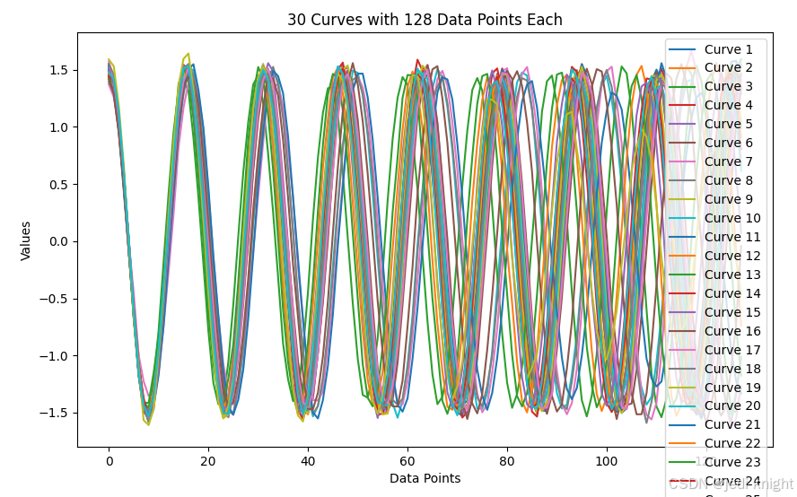
以下是振幅1.5，频率4，相位90度的生成结果，引导系数1.0

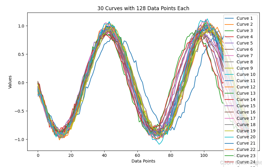
以下是振幅0.8，频率1，相位180度的生成结果，引导系数1.0

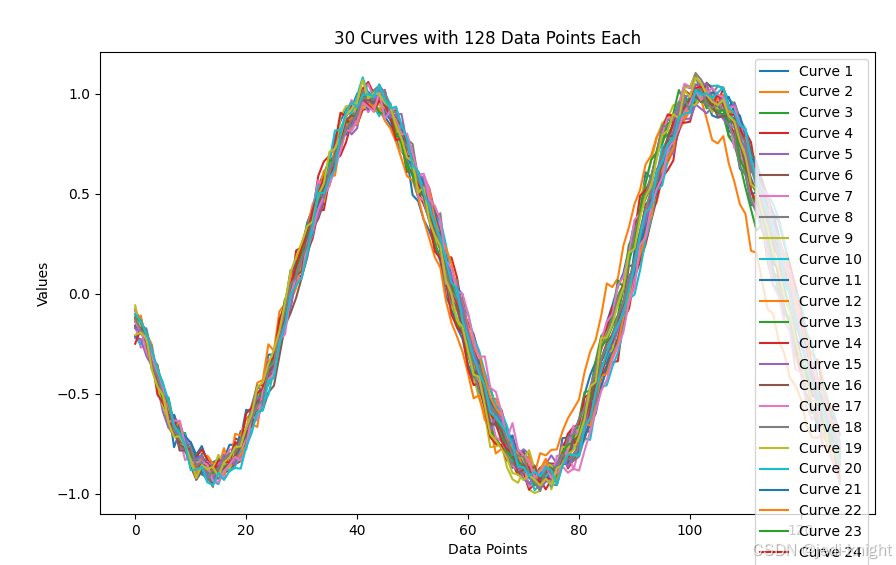
将引导系数扩大为3.0，可以得到更符合条件的结果

将引导系数缩小为0.5，可以得到更多样性的结果

具体应用时，可以通过调整引导系数来控制生成结果的多样性