[机器学习]07-基于多层感知机的鸢尾花数据集分类

• 多类感知机算法：为每个类别学习一个独立的判别函数。通过梯度下降优化权重，使得对每个样本，其真实类别的判别值大于其他类别。

• 决策规则：对测试样本选择判别函数值最大的类别作为预测结果。

程序代码：

import random
import matplotlib
import numpy as np
from matplotlib import pyplot as plt
from sklearn.preprocessing import StandardScalerdata_dict = {}
train_data = {}
test_data = {}matplotlib.rcParams.update({'font.size': 7})with open('Iris数据txt版.txt', 'r') as file:for line in file:line = line.strip()data = line.split('\t')if len(data) >= 3:try:category = data[0]attribute1 = eval(data[1])attribute2 = eval(data[3])if category in ['1', '2', '3']:if category not in data_dict:data_dict[category] = {'Length': [], 'Width': []}data_dict[category]['Length'].append(attribute1)data_dict[category]['Width'].append(attribute2)except ValueError:print(f"Invalid data in line: {line}")continue
for category, attributes in data_dict.items():print(f'种类: {category}')print(len(attributes["Length"]))print(len(attributes["Width"]))print(f'属性1: {attributes["Length"]}')print(f'属性2: {attributes["Width"]}')for category, attributes in data_dict.items():lengths = attributes['Length']widths = attributes['Width']train_indices = random.sample(range(len(lengths)), 45)test_indices = [i for i in range(len(lengths)) if i not in train_indices]train_data[category] = {'Length': [lengths[i] for i in train_indices],'Width': [widths[i] for i in train_indices]}test_data[category] = {'Length': [lengths[i] for i in test_indices],'Width': [widths[i] for i in test_indices]}print(len(train_data['1']['Length']))
print(train_data['1'])
print(len(test_data['1']['Length']))
print(test_data['1'])
print(len(train_data['2']['Length']))
print(train_data['2'])
print(len(test_data['2']['Length']))
print(test_data['2'])
print(len(train_data['3']['Length']))
print(train_data['3'])
print(len(test_data['3']['Length']))
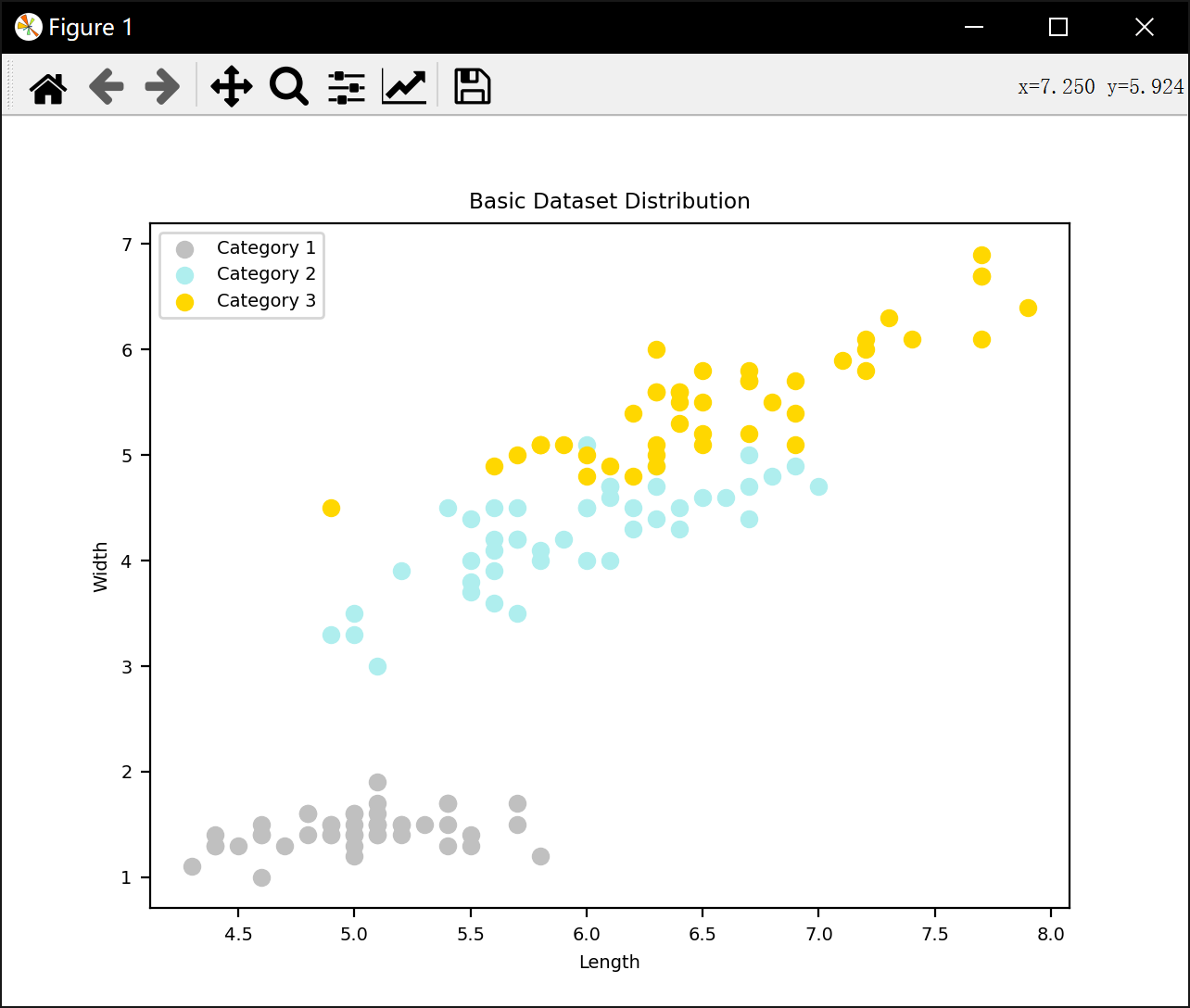
print(test_data['3'])plt.scatter(train_data['1']['Length'], train_data['1']['Width'], color='silver', label='Category 1')
plt.scatter(train_data['2']['Length'], train_data['2']['Width'], color='paleturquoise', label='Category 2')
plt.scatter(train_data['3']['Length'], train_data['3']['Width'], color='gold', label='Category 3')
plt.xlabel('Length')
plt.ylabel('Width')
plt.legend()
plt.title('Basic Dataset Distribution')
plt.show()train_data_merge = []
label_data_merge = []
for category in ['1','2','3']:for i in range(45):attribute1 = train_data[category]['Length'][i]attribute2 = train_data[category]['Width'][i]merged_point = [attribute1, attribute2, 1]train_data_merge.append(merged_point)label_data_merge.append(int(category)-1)#train_data_merge = StandardScaler().fit_transform(train_data_merge)print(train_data_merge)
print(len(train_data_merge))
print(label_data_merge)
print(len(label_data_merge))
lines = np.zeros([3,3])
epochs = 5000
#initial_learning_rate = 0.5
learning_rate_right = 0.5
learning_rate_wrong = 0.5
for i in range(epochs):for j in range(135):for k in range(3):if k != label_data_merge[j]:#print(train_data_merge[category1][j])pright = np.dot(train_data_merge[j], lines[label_data_merge[j]])pwrong = np.dot(train_data_merge[j], lines[k])if pwrong >= pright:gradient_right = np.array(train_data_merge[j])gradient_wrong = np.array(train_data_merge[j])#p_diff = abs(pwrong - pright)#a13_square_sum = sum(x ** 2 for x in gradient_right)#learning_rate_right = initial_learning_rate * p_diff / a13_square_sum#a13_square_sum = sum(x ** 2 for x in gradient_wrong)#learning_rate_wrong = initial_learning_rate * p_diff / a13_square_sum#print(gradient_right,gradient_wrong)lines[label_data_merge[j]] += learning_rate_right * gradient_rightlines[k] -= learning_rate_wrong * gradient_wrong#print(lines[label_data_merge[j]])#print(lines[k])print(lines)
min_x = min(min(train_data['1']['Length']), min(train_data['2']['Length']), min(train_data['3']['Length']))
max_x = max(max(train_data['1']['Length']), max(train_data['2']['Length']), max(train_data['3']['Length']))
x_range = np.linspace(min_x,max_x,int(100*(max_x-min_x)))
k1 = -lines[0][0]/lines[0][1]
k2 = -lines[1][0]/lines[1][1]
k3 = -lines[2][0]/lines[2][1]
b1 = -lines[0][2]/lines[0][1]
b2 = -lines[1][2]/lines[1][1]
b3 = -lines[2][2]/lines[2][1]y_range1 = k1*x_range + b1
y_range2 = k2*x_range + b2
y_range3 = k3*x_range + b3correct_predictions = 0
test_data_merge = []
test_label = []
for category in ['1','2','3']:for i in range(5):attribute1 = test_data[category]['Length'][i]attribute2 = test_data[category]['Width'][i]merged_point = [attribute1, attribute2]test_data_merge.append(merged_point)test_label.append(int(category)-1)# 计算判别函数的值，并分类
for category in ['1', '2', '3']:for i in range(5):attribute1 = test_data[category]['Length'][i]attribute2 = test_data[category]['Width'][i]discriminant_values = []for line in lines:discriminant_value = line[0] * attribute1 + line[1] * attribute2 + line[2]discriminant_values.append(discriminant_value)predicted_category = np.argmax(discriminant_values) + 1if predicted_category == int(category):correct_predictions += 1accuracy = correct_predictions / (5 * 3)
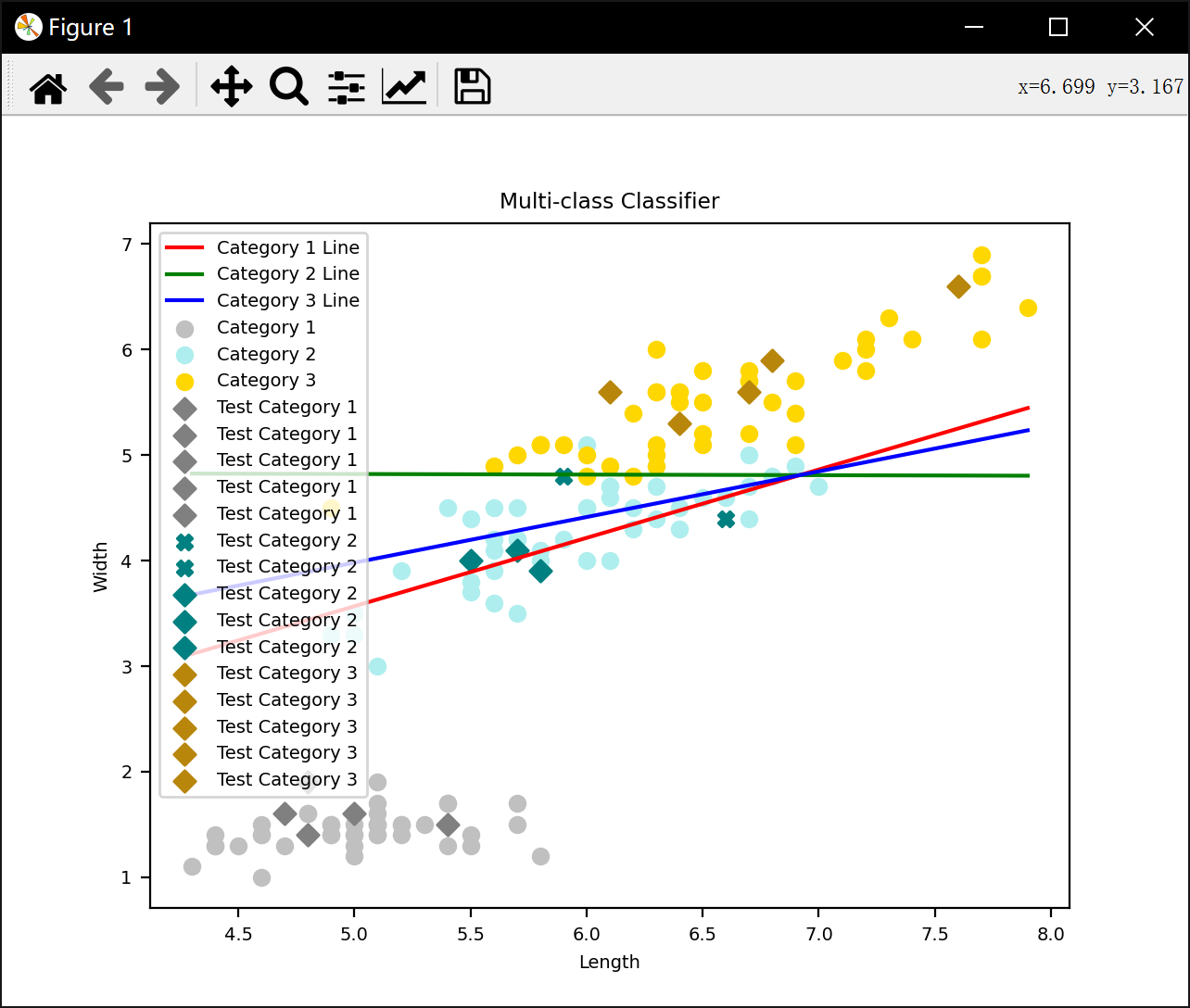
print(f"准确率: {accuracy:.2f}%")plt.plot(x_range, y_range1, color='r', label='Category 1 Line')
plt.plot(x_range, y_range2, color='g', label='Category 2 Line')
plt.plot(x_range, y_range3, color='b', label='Category 3 Line')plt.scatter(train_data['1']['Length'], train_data['1']['Width'], color='silver', label='Category 1')
plt.scatter(train_data['2']['Length'], train_data['2']['Width'], color='paleturquoise', label='Category 2')
plt.scatter(train_data['3']['Length'], train_data['3']['Width'], color='gold', label='Category 3')for i in range(len(test_data_merge)):attribute1 = test_data_merge[i][0]attribute2 = test_data_merge[i][1]true_label = test_label[i]# 计算判别函数的值discriminant_values = []for line in lines:discriminant_value = line[0] * attribute1 + line[1] * attribute2 + line[2]discriminant_values.append(discriminant_value)# 预测的类别predicted_category = np.argmax(discriminant_values) + 1# 根据预测是否正确选择标记形状和颜色marker = 'D' if predicted_category == true_label + 1 else 'X'color = ['gray', 'teal', 'darkgoldenrod'][true_label]plt.scatter(attribute1, attribute2, color=color, label=f'Test Category {true_label + 1}', marker=marker)plt.xlabel('Length')
plt.ylabel('Width')
plt.legend()
plt.title('Multi-class Classifier')
plt.show()

运行结果：

种类: 1
50
50
属性1: [5.1, 4.9, 4.7, 4.6, 5.0, 5.4, 4.6, 5.0, 4.4, 4.9, 5.4, 4.8, 4.8, 4.3, 5.8, 5.7, 5.4, 5.1, 5.7, 5.1, 5.4, 5.1, 4.6, 5.1, 4.8, 5.0, 5.0, 5.2, 5.2, 4.7, 4.8, 5.4, 5.2, 5.5, 4.9, 5.0, 5.5, 4.9, 4.4, 5.1, 5.0, 4.5, 4.4, 5.0, 5.1, 4.8, 5.1, 4.6, 5.3, 5.0]
属性2: [1.4, 1.4, 1.3, 1.5, 1.4, 1.7, 1.4, 1.5, 1.4, 1.5, 1.5, 1.6, 1.4, 1.1, 1.2, 1.5, 1.3, 1.4, 1.7, 1.5, 1.7, 1.5, 1.0, 1.7, 1.9, 1.6, 1.6, 1.5, 1.4, 1.6, 1.6, 1.5, 1.5, 1.4, 1.5, 1.2, 1.3, 1.4, 1.3, 1.5, 1.3, 1.3, 1.3, 1.6, 1.9, 1.4, 1.6, 1.4, 1.5, 1.4]
种类: 2
50
50
属性1: [7.0, 6.4, 6.9, 5.5, 6.5, 5.7, 6.3, 4.9, 6.6, 5.2, 5.0, 5.9, 6.0, 6.1, 5.6, 6.7, 5.6, 5.8, 6.2, 5.6, 5.9, 6.1, 6.3, 6.1, 6.4, 6.6, 6.8, 6.7, 6.0, 5.7, 5.5, 5.5, 5.8, 6.0, 5.4, 6.0, 6.7, 6.3, 5.6, 5.5, 5.5, 6.1, 5.8, 5.0, 5.6, 5.7, 5.7, 6.2, 5.1, 5.7]
属性2: [4.7, 4.5, 4.9, 4.0, 4.6, 4.5, 4.7, 3.3, 4.6, 3.9, 3.5, 4.2, 4.0, 4.7, 3.6, 4.4, 4.5, 4.1, 4.5, 3.9, 4.8, 4.0, 4.9, 4.7, 4.3, 4.4, 4.8, 5.0, 4.5, 3.5, 3.8, 3.7, 3.9, 5.1, 4.5, 4.5, 4.7, 4.4, 4.1, 4.0, 4.4, 4.6, 4.0, 3.3, 4.2, 4.2, 4.2, 4.3, 3.0, 4.1]
种类: 3
50
50
属性1: [6.3, 5.8, 7.1, 6.3, 6.5, 7.6, 4.9, 7.3, 6.7, 7.2, 6.5, 6.4, 6.8, 5.7, 5.8, 6.4, 6.5, 7.7, 7.7, 6.0, 6.9, 5.6, 7.7, 6.3, 6.7, 7.2, 6.2, 6.1, 6.4, 7.2, 7.4, 7.9, 6.4, 6.3, 6.1, 7.7, 6.3, 6.4, 6.0, 6.9, 6.7, 6.9, 5.8, 6.8, 6.7, 6.7, 6.3, 6.5, 6.2, 5.9]
属性2: [6.0, 5.1, 5.9, 5.6, 5.8, 6.6, 4.5, 6.3, 5.8, 6.1, 5.1, 5.3, 5.5, 5.0, 5.1, 5.3, 5.5, 6.7, 6.9, 5.0, 5.7, 4.9, 6.7, 4.9, 5.7, 6.0, 4.8, 4.9, 5.6, 5.8, 6.1, 6.4, 5.6, 5.1, 5.6, 6.1, 5.6, 5.5, 4.8, 5.4, 5.6, 5.1, 5.1, 5.9, 5.7, 5.2, 5, 5.2, 5.4, 5.1]
45
{'Length': [4.4, 4.8, 5.1, 5.4, 5.2, 4.3, 5.1, 5.2, 5.0, 5.1, 5.1, 4.6, 5.7, 5.0, 4.5, 4.6, 4.8, 5.8, 4.4, 4.9, 5.4, 5.0, 5.2, 5.7, 5.5, 5.1, 4.4, 5.3, 5.0, 5.4, 5.0, 4.8, 4.7, 5.4, 5.5, 5.0, 4.6, 5.1, 4.9, 5.1, 4.9, 5.0, 4.6, 4.9, 5.1], 'Width': [1.3, 1.4, 1.7, 1.5, 1.5, 1.1, 1.4, 1.4, 1.4, 1.6, 1.5, 1.5, 1.7, 1.6, 1.3, 1.0, 1.6, 1.2, 1.4, 1.4, 1.3, 1.3, 1.5, 1.5, 1.3, 1.5, 1.3, 1.5, 1.5, 1.7, 1.4, 1.6, 1.3, 1.7, 1.4, 1.6, 1.4, 1.4, 1.4, 1.9, 1.5, 1.2, 1.4, 1.5, 1.5]}
5
{'Length': [5.4, 4.8, 4.8, 4.7, 5.0], 'Width': [1.5, 1.4, 1.9, 1.6, 1.6]}
45
{'Length': [6.1, 5.4, 5.7, 6.2, 5.2, 6.7, 5.7, 6.5, 6.4, 6.4, 6.7, 6.3, 6.7, 6.3, 5.5, 6.8, 5.7, 5.6, 5.9, 6.2, 5.6, 5.0, 6.3, 5.5, 5.8, 6.0, 5.1, 6.1, 4.9, 6.6, 6.0, 6.1, 5.0, 5.5, 5.8, 5.6, 5.6, 5.5, 7.0, 6.0, 6.0, 6.1, 5.7, 5.6, 6.9], 'Width': [4.7, 4.5, 4.5, 4.5, 3.9, 4.7, 4.2, 4.6, 4.5, 4.3, 4.4, 4.9, 5.0, 4.7, 4.4, 4.8, 3.5, 4.5, 4.2, 4.3, 4.2, 3.3, 4.4, 3.7, 4.0, 4.5, 3.0, 4.6, 3.3, 4.6, 4.0, 4.0, 3.5, 3.8, 4.1, 4.1, 3.9, 4.0, 4.7, 4.5, 5.1, 4.7, 4.2, 3.6, 4.9]}
5
{'Length': [5.9, 6.6, 5.8, 5.5, 5.7], 'Width': [4.8, 4.4, 3.9, 4.0, 4.1]}
45
{'Length': [7.2, 7.9, 7.7, 6.3, 6.1, 5.7, 6.4, 6.0, 6.3, 6.0, 6.3, 7.7, 7.3, 6.5, 5.6, 7.1, 7.7, 5.8, 5.8, 6.5, 6.2, 6.2, 6.4, 6.7, 6.4, 6.7, 5.9, 6.3, 4.9, 7.4, 7.2, 6.9, 6.5, 7.7, 5.8, 6.8, 6.4, 6.3, 7.2, 6.5, 6.7, 6.9, 6.7, 6.9, 6.3], 'Width': [6.0, 6.4, 6.7, 5.1, 4.9, 5.0, 5.6, 4.8, 4.9, 5.0, 5, 6.7, 6.3, 5.8, 4.9, 5.9, 6.9, 5.1, 5.1, 5.5, 5.4, 4.8, 5.3, 5.7, 5.6, 5.8, 5.1, 5.6, 4.5, 6.1, 5.8, 5.7, 5.2, 6.1, 5.1, 5.5, 5.5, 5.6, 6.1, 5.1, 5.7, 5.1, 5.2, 5.4, 6.0]}
5
{'Length': [7.6, 6.4, 6.1, 6.7, 6.8], 'Width': [6.6, 5.3, 5.6, 5.6, 5.9]}
[[4.4, 1.3, 1], [4.8, 1.4, 1], [5.1, 1.7, 1], [5.4, 1.5, 1], [5.2, 1.5, 1], [4.3, 1.1, 1], [5.1, 1.4, 1], [5.2, 1.4, 1], [5.0, 1.4, 1], [5.1, 1.6, 1], [5.1, 1.5, 1], [4.6, 1.5, 1], [5.7, 1.7, 1], [5.0, 1.6, 1], [4.5, 1.3, 1], [4.6, 1.0, 1], [4.8, 1.6, 1], [5.8, 1.2, 1], [4.4, 1.4, 1], [4.9, 1.4, 1], [5.4, 1.3, 1], [5.0, 1.3, 1], [5.2, 1.5, 1], [5.7, 1.5, 1], [5.5, 1.3, 1], [5.1, 1.5, 1], [4.4, 1.3, 1], [5.3, 1.5, 1], [5.0, 1.5, 1], [5.4, 1.7, 1], [5.0, 1.4, 1], [4.8, 1.6, 1], [4.7, 1.3, 1], [5.4, 1.7, 1], [5.5, 1.4, 1], [5.0, 1.6, 1], [4.6, 1.4, 1], [5.1, 1.4, 1], [4.9, 1.4, 1], [5.1, 1.9, 1], [4.9, 1.5, 1], [5.0, 1.2, 1], [4.6, 1.4, 1], [4.9, 1.5, 1], [5.1, 1.5, 1], [6.1, 4.7, 1], [5.4, 4.5, 1], [5.7, 4.5, 1], [6.2, 4.5, 1], [5.2, 3.9, 1], [6.7, 4.7, 1], [5.7, 4.2, 1], [6.5, 4.6, 1], [6.4, 4.5, 1], [6.4, 4.3, 1], [6.7, 4.4, 1], [6.3, 4.9, 1], [6.7, 5.0, 1], [6.3, 4.7, 1], [5.5, 4.4, 1], [6.8, 4.8, 1], [5.7, 3.5, 1], [5.6, 4.5, 1], [5.9, 4.2, 1], [6.2, 4.3, 1], [5.6, 4.2, 1], [5.0, 3.3, 1], [6.3, 4.4, 1], [5.5, 3.7, 1], [5.8, 4.0, 1], [6.0, 4.5, 1], [5.1, 3.0, 1], [6.1, 4.6, 1], [4.9, 3.3, 1], [6.6, 4.6, 1], [6.0, 4.0, 1], [6.1, 4.0, 1], [5.0, 3.5, 1], [5.5, 3.8, 1], [5.8, 4.1, 1], [5.6, 4.1, 1], [5.6, 3.9, 1], [5.5, 4.0, 1], [7.0, 4.7, 1], [6.0, 4.5, 1], [6.0, 5.1, 1], [6.1, 4.7, 1], [5.7, 4.2, 1], [5.6, 3.6, 1], [6.9, 4.9, 1], [7.2, 6.0, 1], [7.9, 6.4, 1], [7.7, 6.7, 1], [6.3, 5.1, 1], [6.1, 4.9, 1], [5.7, 5.0, 1], [6.4, 5.6, 1], [6.0, 4.8, 1], [6.3, 4.9, 1], [6.0, 5.0, 1], [6.3, 5, 1], [7.7, 6.7, 1], [7.3, 6.3, 1], [6.5, 5.8, 1], [5.6, 4.9, 1], [7.1, 5.9, 1], [7.7, 6.9, 1], [5.8, 5.1, 1], [5.8, 5.1, 1], [6.5, 5.5, 1], [6.2, 5.4, 1], [6.2, 4.8, 1], [6.4, 5.3, 1], [6.7, 5.7, 1], [6.4, 5.6, 1], [6.7, 5.8, 1], [5.9, 5.1, 1], [6.3, 5.6, 1], [4.9, 4.5, 1], [7.4, 6.1, 1], [7.2, 5.8, 1], [6.9, 5.7, 1], [6.5, 5.2, 1], [7.7, 6.1, 1], [5.8, 5.1, 1], [6.8, 5.5, 1], [6.4, 5.5, 1], [6.3, 5.6, 1], [7.2, 6.1, 1], [6.5, 5.1, 1], [6.7, 5.7, 1], [6.9, 5.1, 1], [6.7, 5.2, 1], [6.9, 5.4, 1], [6.3, 6.0, 1]]
135
[0, 0, 0, 0, 0, 0, 0, 0, 0, 0, 0, 0, 0, 0, 0, 0, 0, 0, 0, 0, 0, 0, 0, 0, 0, 0, 0, 0, 0, 0, 0, 0, 0, 0, 0, 0, 0, 0, 0, 0, 0, 0, 0, 0, 0, 1, 1, 1, 1, 1, 1, 1, 1, 1, 1, 1, 1, 1, 1, 1, 1, 1, 1, 1, 1, 1, 1, 1, 1, 1, 1, 1, 1, 1, 1, 1, 1, 1, 1, 1, 1, 1, 1, 1, 1, 1, 1, 1, 1, 1, 2, 2, 2, 2, 2, 2, 2, 2, 2, 2, 2, 2, 2, 2, 2, 2, 2, 2, 2, 2, 2, 2, 2, 2, 2, 2, 2, 2, 2, 2, 2, 2, 2, 2, 2, 2, 2, 2, 2, 2, 2, 2, 2, 2, 2]
135
[[  58.9   -90.95   30.  ]
[  -0.25  -44.65  216.5 ]
[ -58.65  135.6  -246.5 ]]
准确率: 0.87%

进程已结束,退出代码0