机器学习监督学习实战六:五种算法对新闻组英文文档进行文本分类(20类),词频统计和TF-IDF 转换特征提取方法理论和对比解析
本文主要介绍了20 Newsgroups数据集及其在文本分类任务中的应用。20 Newsgroups数据集包含约20,000篇新闻组文档,分为20个不同主题的新闻组,数据集被分为训练集和测试集。在数据预处理阶段,使用了CountVectorizer和TfidfVectorizer两种方法将文本数据转换为数值特征,最终选择了TF-IDF特征用于模型训练和评估。通过10折交叉验证评估了多种算法的性能,包括逻辑回归(LR)、支持向量机(SVM)、分类与回归树(CART)、多项式朴素贝叶斯(MNB)和K近邻(KNN),其中SVM和LR表现较好。进一步对逻辑回归进行了网格搜索调参准确率达到0.9214%,最终在测试集上验证了调参后的模型准确率,并生成了分类报告。完整代码已开源在个人GitHub:https://github.com/KLWU07/Text-classification-of-newsgroup-documents
一、数据集介绍
1.数据集来源与构成
20 Newsgroups 数据集收集了大约 20,000 左右的新闻组文档,均匀分为 20 个不同主题的新闻组集合。 20news - bydate - train 和 20news - bydate - test 来自 20 Newsgroups 数据集的 bydate 版本,该版本按时间顺序将数据集分为训练集(约占 60%)和测试集(约占 40%),不包含重复文档和新闻组名,共包含 18,846 个文档。数据集信息来自于https://archive.ics.uci.edu/dataset/113/twenty+newsgroups,可下载。
2.数据特点
- 分类多样:涵盖计算机技术、体育、政治、宗教等 20 个不同的主题。
- 高维度:每篇文章都是由大量的单词组成。
3.类别信息
1.计算机技术相关
comp.graphics
主题:计算机图形学、图像渲染、图形软件等(如 OpenGL、3D 建模)。
comp.os.ms-windows.misc
主题:Windows 操作系统相关问题、软件使用、系统故障等。
comp.sys.ibm.pc.hardware
主题:IBM PC 硬件(如主板、显卡、硬盘等硬件故障与配置)。
comp.sys.mac.hardware
主题:苹果 Mac 硬件(如 Mac 电脑、配件、性能优化等)。
comp.windows.x
主题:Windows 系统下的 X 窗口系统(如图形界面开发、X11 配置等)。2.科学与学术相关
sci.astro
主题:天文学、宇宙学、天文观测、星系研究等。
sci.crypt
主题:密码学、加密算法、安全协议、区块链技术(早期相关讨论)等。
sci.electronics
主题:电子工程、电路设计、半导体技术、电子元件等。
sci.med
主题:医学研究、疾病诊断、生物技术、医疗设备等(非临床实践,偏学术)。
sci.space
主题:航天工程、太空探索、卫星技术、星际旅行等。3.娱乐与社会文化
rec.autos
主题:汽车爱好、车型讨论、汽车改装、赛车运动等。
rec.motorcycles
主题:摩托车爱好、摩托车型号、骑行体验、摩托车赛事等。
rec.sport.hockey
主题:冰球运动(如 NHL 赛事、规则讨论、球员动态等)。
rec.sport.baseball
主题:棒球运动(如 MLB 赛事、战术分析、球员数据等)。
misc.forsale
主题:二手交易、商品出售、拍卖信息、商业广告等(综合性分类)。4.政治与宗教
talk.politics.misc
主题:综合政治话题(如政策辩论、选举分析、国际关系等)。
talk.politics.guns
主题:美国枪支政策、枪械权利、控枪辩论等。
talk.politics.mideast
主题:中东政治(如地区冲突、宗教矛盾、国际关系等)。
talk.religion.misc
主题:综合宗教讨论(如信仰比较、神学争议、宗教节日等)。
alt.atheism
主题:无神论、宗教批判、哲学讨论(与宗教相关的非信仰观点)。
4.其中一个文档样本展示
From: MJMUISE@1302.watstar.uwaterloo.ca (Mike Muise)
Subject: Re: Drinking and Riding    %% 主题 :回复:饮酒与骑行
Lines: 19 							%% 行数 :19
Organization: Waterloo Engineering  %% 组织 :滑铁卢工程学院In article <C4wKBp.B9w@eskimo.com>, maven@eskimo.com (Norman Hamer) writes:
>  What is a general rule of thumb for sobriety and cycling? Couple hours
> after you "feel" sober? What? Or should I just work with "If I drink
> tonight, I don't ride until tomorrow"?
%% 醒酒和骑自行车的一般经验法则是什么?在你“感觉”清醒后几个小时?是什么?还是我应该坚持“如果我今晚喝酒,我就等到明天再骑车”?1 hr/drink for the first 4 drinks.       %% 前4杯酒,每杯酒1小时。
1.5 hours/drink for the next 6 drinks.   %% 接下来的6杯酒,每杯酒1.5小时。
2 hours/drink for the rest.				 %% 其余的酒,每杯酒2小时。These are fairly cautious guidelines, and will work even if you happen to
have a low tolerance or body mass.
I think the cops and "Don't You Dare Drink & Drive" (tm) commercials will
usually say 1hr/drink in general, but after about 5 drinks and 5 hrs, you
could very well be over the legal limit.
Watch yourself.
%% 这些是比较谨慎的指导方针,即使你碰巧酒量低或者体重轻,也适用。
我认为警察和“不要酒后驾车”(商标)广告通常会说一般每杯酒1小时,但喝了大约5杯酒并且过了5小时后,你很可能仍然超过法定限度。
注意自己。-Mike________________________________________________/ Mike Muise / mjmuise@1302.watstar.uwaterloo.ca \ no quotes, no jokes,\ Electrical Engineering, University of Waterloo / no disclaimer, no fear.
二、文件特征提取(数据预处理)
这是自然语言处理(NLP)中处理文本数据的经典流程,用于将非结构化文本转换为机器学习模型可处理的数值特征。两种方法都有调用,代码中同时使用了 CountVectorizer 和 TfidfVectorizer,但最终只使用了 TF-IDF 特征(即 X_train_counts_tf)进行模型训练和评估。
| 方法 | CountVectorizer | TfidfVectorizer |
|---|---|---|
| 核心思想 | 统计词汇在文本中出现的次数 | 评估词汇对文本的区分能力(词频 × 逆文档频率) |
| 权重计算 | 每个词的权重 = 出现次数 | 每个词的权重 = TF × IDF |
| 对高频词的处理 | 无处理(所有词平等对待) | 抑制通用高频词(如 “the”),提升稀有词权重 |
| 特征矩阵特点 | 数值非负,可能存在大量重复值 | 数值范围更广,重要词权重更高 |
| 文本分类 | 适用于短文本、词汇分布均匀的场景 | 通常表现更好,尤其在长文本、多类别场景 |
| 垃圾邮件检测 | 可能被 “buy”“free” 等高频词误导 | 能有效识别低频但关键的垃圾词模式 |
| 主题模型(如 LDA) | 直接使用词频更符合概率模型假设 | 可能因权重调整导致主题偏移 |
| 计算效率 | 更快(仅需计数) | 稍慢(需额外计算 IDF) |
| 特征稀疏性 | 更高(大量零值) | 相对较低(重要词权重更突出) |
1. 词频统计(CountVectorizer)
词频统计:使用CountVectorizer计算词频矩阵。
stop_words='english'
- 自动过滤英语停用词(如 “the”, “and”, “is” 等无实际语义的高频词),减少噪声特征。
decode_error='ignore'
- 忽略无法解码的字符(如乱码),确保文本处理的鲁棒性。
fit_transform()
- 训练(fit):分析所有文本,构建词汇表(如{“apple”: 0, “banana”: 1, …})。
- 转换(transform):将每篇文本转换为向量,向量维度等于词汇表大小,每个位置的值表示对应词汇在文本中的出现次数。
2.TF-IDF 转换(TfidfVectorizer)
- TF-IDF 转换:将词频矩阵转换为 TF-IDF(词频 - 逆文档频率)矩阵,突出重要词汇的权重。
- TF-IDF(Term Frequency-Inverse Document Frequency)是一种统计方法,用于评估词汇在文本集合中的重要性。
- 词频(TF):词汇在单个文本中出现的频率。
公式:TF = 词汇在文本中出现次数 / 文本总词数 - 逆文档频率(IDF):衡量词汇的普遍重要性(若某词在所有文本中频繁出现,则重要性低)。
公式:IDF = log(总文档数 / 包含该词的文档数 + 1) - TF-IDF 值:TF × IDF,值越高表示词汇对文本的区分能力越强。
3.词频统计的局限性
- 维度灾难:词汇表可能包含数万甚至数十万个词,导致特征矩阵维度极高。
- 噪声问题:高频词(如 “the”)对分类无帮助,但会占据大量特征空间。
4.TF-IDF 的优势
- 特征降维:通过权重调整,弱化普遍词汇,突出有区分性的词汇。
- 语义增强:提升与类别相关的关键词(如在 “comp.graphics” 类别中,“pixel” 的 TF-IDF 值会更高)的权重。
5.特征扩展
- 词嵌入(Word Embedding):使用 Word2Vec、GloVe 等方法捕捉词汇语义关系(优于 TF-IDF 的词袋模型)。
- 文本预处理:结合词干提取(Stemming)或词形还原(Lemmatization)进一步减少特征维度。
6.CountVectorizer和TF-IDF()举例比较
对比还是不一样的。
from sklearn.feature_extraction.text import CountVectorizer
from sklearn.feature_extraction.text import TfidfVectorizershili = ['What is a general rule of thumb for sobriety and cycling? Couple hours after you "feel" sober? What? Or should I just work with "If I drink tonight, I do not ride until tomorrow"? ','1 hour drink for the first 4 drinks.','1.5 hours drink for the next 6 drinks.','2 hours drink for the rest.'
]tz = CountVectorizer()
tz1 = CountVectorizer(stop_words='english', decode_error='ignore')
X = tz.fit_transform(shili)
X1 = tz.fit_transform(shili)print(X.shape,X1.shape)
print(X.toarray(),'\n\n',X1.toarray())
print('-'*100)
tz3 = TfidfVectorizer()
Y1 = tz3.fit_transform(shili)tz4 = TfidfVectorizer(stop_words='english', decode_error='ignore')
Y2 = tz4.fit_transform(shili)
print(Y1.shape,Y2.shape)
print(Y1.toarray(),'\n\n',Y2.toarray())
(4, 35) (4, 35)
[[1 1 1 1 1 1 0 1 0 1 1 0 1 1 1 1 0 1 1 1 0 1 1 1 1 1 0 1 1 1 1 2 1 1 1][0 0 0 0 0 1 1 0 1 1 0 1 0 0 0 0 0 0 0 0 0 0 0 0 0 0 1 0 0 0 0 0 0 0 0][0 0 0 0 0 1 1 0 0 1 0 0 1 0 0 0 1 0 0 0 0 0 0 0 0 0 1 0 0 0 0 0 0 0 0][0 0 0 0 0 1 0 0 0 1 0 0 1 0 0 0 0 0 0 0 1 0 0 0 0 0 1 0 0 0 0 0 0 0 0]] [[1 1 1 1 1 1 0 1 0 1 1 0 1 1 1 1 0 1 1 1 0 1 1 1 1 1 0 1 1 1 1 2 1 1 1][0 0 0 0 0 1 1 0 1 1 0 1 0 0 0 0 0 0 0 0 0 0 0 0 0 0 1 0 0 0 0 0 0 0 0][0 0 0 0 0 1 1 0 0 1 0 0 1 0 0 0 1 0 0 0 0 0 0 0 0 0 1 0 0 0 0 0 0 0 0][0 0 0 0 0 1 0 0 0 1 0 0 1 0 0 0 0 0 0 0 1 0 0 0 0 0 1 0 0 0 0 0 0 0 0]]
----------------------------------------------------------------------------------------------------
(4, 35) (4, 18)
[[0.18272028 0.18272028 0.18272028 0.18272028 0.18272028 0.095351020.         0.18272028 0.         0.09535102 0.18272028 0.0.11662799 0.18272028 0.18272028 0.18272028 0.         0.182720280.18272028 0.18272028 0.         0.18272028 0.18272028 0.182720280.18272028 0.18272028 0.         0.18272028 0.18272028 0.182720280.18272028 0.36544055 0.18272028 0.18272028 0.18272028][0.         0.         0.         0.         0.         0.27604710.41705904 0.         0.52898651 0.2760471  0.         0.528986510.         0.         0.         0.         0.         0.0.         0.         0.         0.         0.         0.0.         0.         0.33764523 0.         0.         0.0.         0.         0.         0.         0.        ][0.         0.         0.         0.         0.         0.302241390.45663404 0.         0.         0.30224139 0.         0.0.36968461 0.         0.         0.         0.57918237 0.0.         0.         0.         0.         0.         0.0.         0.         0.36968461 0.         0.         0.0.         0.         0.         0.         0.        ][0.         0.         0.         0.         0.         0.33972890.         0.         0.         0.3397289  0.         0.0.41553722 0.         0.         0.         0.         0.0.         0.         0.65101935 0.         0.         0.0.         0.         0.41553722 0.         0.         0.0.         0.         0.         0.         0.        ]] [[0.27037171 0.27037171 0.14109118 0.         0.27037171 0.270371710.         0.17257476 0.27037171 0.         0.27037171 0.270371710.27037171 0.27037171 0.27037171 0.27037171 0.27037171 0.27037171][0.         0.         0.37919167 0.5728925  0.         0.0.72664149 0.         0.         0.         0.         0.0.         0.         0.         0.         0.         0.        ][0.         0.         0.4574528  0.69113141 0.         0.0.         0.55953044 0.         0.         0.         0.0.         0.         0.         0.         0.         0.        ][0.         0.         0.40264194 0.         0.         0.0.         0.49248889 0.         0.77157901 0.         0.0.         0.         0.         0.         0.         0.        ]]
三、算法评估
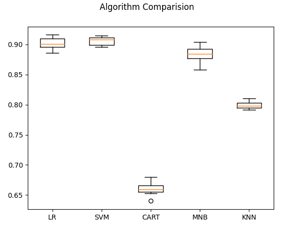
1.10折交叉验证和准确率(箱线图)
实际加载的类别数: 20
类别名称: ['alt.atheism', 'comp.graphics', 'comp.os.ms-windows.misc', 'comp.sys.ibm.pc.hardware', 'comp.sys.mac.hardware', 'comp.windows.x', 'misc.forsale', 'rec.autos', 'rec.motorcycles', 'rec.sport.baseball', 'rec.sport.hockey', 'sci.crypt', 'sci.electronics', 'sci.med', 'sci.space', 'soc.religion.christian', 'talk.politics.guns', 'talk.politics.mideast', 'talk.politics.misc', 'talk.religion.misc']
(11314, 129782)
(11314, 129782)
LR : 0.902158 (0.008985)
SVM : 0.905958 (0.006622)
CART : 0.660421 (0.010269)
MNB : 0.883951 (0.012686)
KNN : 0.799187 (0.006339)
2.逻辑回归LR网格搜索GridSearchCV
# 4)算法调参
# 调参LR
param_grid = {}
param_grid['C'] = [0.1, 5, 13, 15]
model = LogisticRegression(C=13, max_iter=1000)
kfold = KFold(n_splits=num_folds,shuffle=True, random_state=seed)
grid = GridSearchCV(estimator=model, param_grid=param_grid, scoring=scoring, cv=kfold)
grid_result = grid.fit(X=X_train_counts_tf, y=dataset_train.target)
print('最优 : %s 使用 %s' % (grid_result.best_score_, grid_result.best_params_))
最优 : 0.9214261277895981 使用 {'C': 15}
3.验证集验证准确率
# 6)生成模型
model = LogisticRegression(C=15)
model.fit(X_train_counts_tf, dataset_train.target)
X_test_counts = tf_transformer.transform(dataset_test.data)
predictions = model.predict(X_test_counts)
print(accuracy_score(dataset_test.target, predictions))
print(classification_report(dataset_test.target, predictions))
0.846388741370154precision    recall  f1-score   support0       0.82      0.77      0.79       3191       0.73      0.81      0.77       3892       0.77      0.75      0.76       3943       0.71      0.75      0.73       3924       0.82      0.85      0.84       3855       0.84      0.76      0.80       3956       0.80      0.89      0.84       3907       0.92      0.90      0.91       3968       0.96      0.95      0.96       3989       0.91      0.94      0.92       39710       0.96      0.97      0.96       39911       0.96      0.92      0.94       39612       0.78      0.79      0.78       39313       0.90      0.87      0.88       39614       0.91      0.92      0.91       39415       0.86      0.93      0.89       39816       0.75      0.90      0.82       36417       0.98      0.89      0.93       37618       0.82      0.61      0.70       31019       0.73      0.61      0.66       251accuracy                           0.85      7532macro avg       0.85      0.84      0.84      7532
weighted avg       0.85      0.85      0.85      7532
四、完整代码
from sklearn.datasets import load_files
from sklearn.feature_extraction.text import TfidfVectorizer
from sklearn.linear_model import LogisticRegression
from sklearn.model_selection import cross_val_score
from sklearn.model_selection import KFold
from joblib import dump, load  # 导入模型保存和加载的函数# 1) 导入数据
categories = ['alt.atheism','rec.sport.hockey','comp.graphics','sci.crypt','comp.os.ms-windows.misc','sci.electronics','comp.sys.ibm.pc.hardware','sci.med','comp.sys.mac.hardware','sci.space','comp.windows.x','soc.religion.christian','misc.forsale','talk.politics.guns','rec.autos','talk.politics.mideast','rec.motorcycles','talk.politics.misc','rec.sport.baseball','talk.religion.misc']
# 导入训练数据
train_path = '20news-bydate-train'
dataset_train = load_files(container_path=train_path, categories=categories)
# 导入评估数据
test_path = '20news-bydate-test'
dataset_test = load_files(container_path=test_path, categories=categories)print("实际加载的类别数:", len(dataset_train.target_names))
print("类别名称:", dataset_train.target_names)# 计算TF-IDF
tf_transformer = TfidfVectorizer(stop_words='english', decode_error='ignore')
X_train_counts_tf = tf_transformer.fit_transform(dataset_train.data)
# 查看数据维度
print(X_train_counts_tf.shape)# 保存TF-IDF向量器
dump(tf_transformer, 'tfidf_vectorizer.joblib')# 设置评估算法的基准
num_folds = 10
seed = 7
scoring = 'accuracy'# 生成算法模型
models = {}
models['LR'] = LogisticRegression(C=15,n_jobs=-1, max_iter=1000)# 比较算法
results = []
for key in models:kfold = KFold(n_splits=num_folds, shuffle=True, random_state=seed)cv_results = cross_val_score(models[key], X_train_counts_tf, dataset_train.target, cv=kfold, scoring=scoring)results.append(cv_results)print('%s : %f (%f)' % (key, cv_results.mean(), cv_results.std()))# 训练完整模型(不使用交叉验证)model = models[key]model.fit(X_train_counts_tf, dataset_train.target)# 保存模型model_filename = f'{key}_model.joblib'dump(model, model_filename)print(f'模型已保存为 {model_filename}')# 保存类别名称
dump(dataset_train.target_names, 'target_names.joblib')
五.预测
GPT随机汽车发布会的邮件——car _txt文本格式。
from joblib import load# 加载组件
tf_transformer = load('tfidf_vectorizer.joblib')  # 加载TF-IDF向量化器
model = load('LR_model.joblib')                   # 加载训练好的模型
target_names = load('target_names.joblib')        # 加载类别名称# 1. 读取 `txt` 文件内容
file_path = 'car_1.txt'  # 确保文件路径正确
with open(file_path, 'r', encoding='utf-8', errors='ignore') as f:text = f.read()# 2. 向量化文本
X_new = tf_transformer.transform([text])  # 注意:输入必须是列表形式(即使单样本)print(X_new.shape)
print(X_new.toarray())
# 3. 预测类别
predicted = model.predict(X_new)
predicted_class = target_names[predicted[0]]  # 获取类别名称# 4. 输出结果
print(f"文件 '{file_path}' 的预测类别是: {predicted_class}")
(1, 129782)
[[0. 0. 0. ... 0. 0. 0.]]
文件 'car_1.txt' 的预测类别是: rec.autos