DAY9 热力图和箱线图的绘制
浙大疏锦行
学会了绘制两个图:
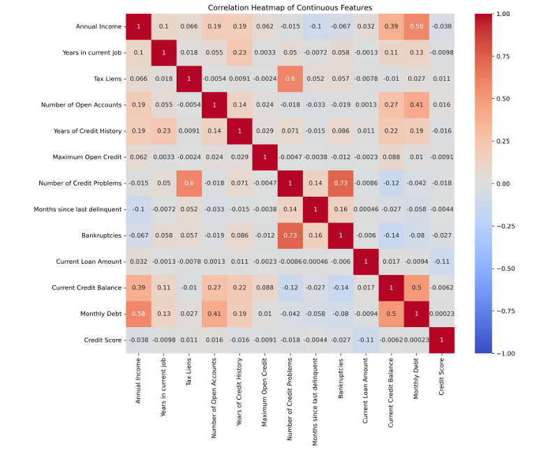
热力图:表示每个特征之间的影响,颜色越深数值越大表示这两个特征的关系越紧密
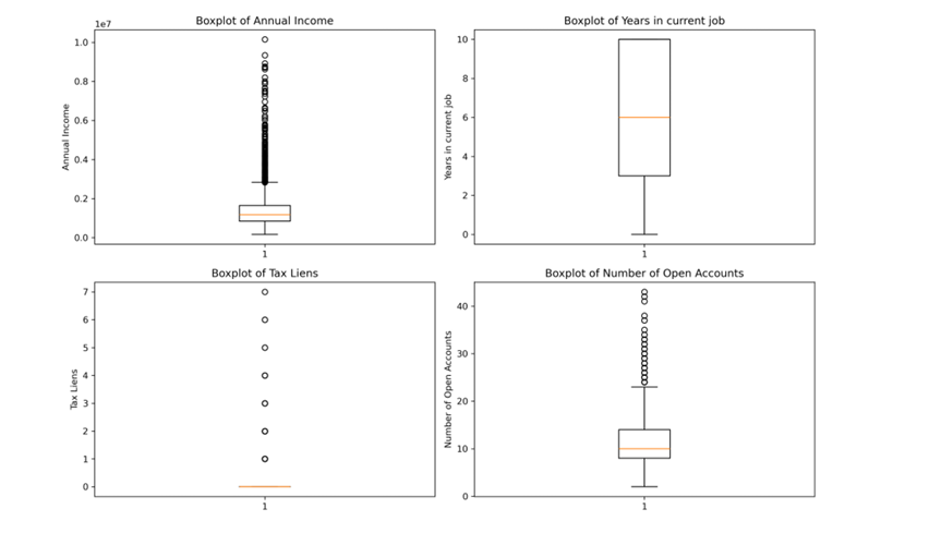
箱线图:表示每个特征的数据分布情况
箱体(Box):
箱体的上下边界分别表示第一四分位数(Q1)和第三四分位数(Q3),即数据的25%和75%分位数。
箱体内的水平线表示中位数(Median),即数据的50%分位数。
须(Whiskers):
须的上下端点通常表示数据的最小值和最大值,但不包括异常值。
在这个图中,须的下端点接近0,上端点大约在200,000左右。
异常值(Outliers):
图中箱体外的圆点表示异常值,即显著偏离其他数据点的值。
在这个图中,可以看到许多异常值,这些值远高于第三四分位数(Q3)。
数据分布:
从图中可以看出,年收入的中位数较低,大部分数据集中在较低的收入范围内。
然而,存在一些高收入的异常值,这些值显著高于大多数数据点
# 首先走一遍完整的之前的流程
# 1. 读取数据
import pandas as pd
data  = pd.read_csv('data.csv')
# 2. 查看数据
data.info()
<class 'pandas.core.frame.DataFrame'>
RangeIndex: 7500 entries, 0 to 7499
Data columns (total 18 columns):#   Column                        Non-Null Count  Dtype
---  ------                        --------------  -----  0   Id                            7500 non-null   int64  1   Home Ownership                7500 non-null   object 2   Annual Income                 5943 non-null   float643   Years in current job          7129 non-null   object 4   Tax Liens                     7500 non-null   float645   Number of Open Accounts       7500 non-null   float646   Years of Credit History       7500 non-null   float647   Maximum Open Credit           7500 non-null   float648   Number of Credit Problems     7500 non-null   float649   Months since last delinquent  3419 non-null   float6410  Bankruptcies                  7486 non-null   float6411  Purpose                       7500 non-null   object 12  Term                          7500 non-null   object 13  Current Loan Amount           7500 non-null   float6414  Current Credit Balance        7500 non-null   float6415  Monthly Debt                  7500 non-null   float6416  Credit Score                  5943 non-null   float6417  Credit Default                7500 non-null   int64
dtypes: float64(12), int64(2), object(4)
memory usage: 1.0+ MB
data["Years in current job"].value_counts()Years in current job
10+ years 2332
2 years 705
3 years 620
< 1 year 563
5 years 516
1 year 504
4 years 469
6 years 426
7 years 396
8 years 339
9 years 259
Name: count, dtype: int64
data["Home Ownership"].value_counts()
Home Ownership
Home Mortgage    3637
Rent             3204
Own Home          647
Have Mortgage      12
Name: count, dtype: int64
# 创建嵌套字典用于映射
mappings = {"Years in current job": {"10+ years": 10,"2 years": 2,"3 years": 3,"< 1 year": 0,"5 years": 5,"1 year": 1,"4 years": 4,"6 years": 6,"7 years": 7,"8 years": 8,"9 years": 9},"Home Ownership": {"Home Mortgage": 0,"Rent": 1,"Own Home": 2,"Have Mortgage": 3}
}
# 使用映射字典进行转换
data["Years in current job"] = data["Years in current job"].map(mappings["Years in current job"])
data["Home Ownership"] = data["Home Ownership"].map(mappings["Home Ownership"])
data.info()
<class 'pandas.core.frame.DataFrame'>
RangeIndex: 7500 entries, 0 to 7499
Data columns (total 18 columns):#   Column                        Non-Null Count  Dtype
---  ------                        --------------  -----  0   Id                            7500 non-null   int64  1   Home Ownership                7500 non-null   int64  2   Annual Income                 5943 non-null   float643   Years in current job          7129 non-null   float644   Tax Liens                     7500 non-null   float645   Number of Open Accounts       7500 non-null   float646   Years of Credit History       7500 non-null   float647   Maximum Open Credit           7500 non-null   float648   Number of Credit Problems     7500 non-null   float649   Months since last delinquent  3419 non-null   float6410  Bankruptcies                  7486 non-null   float6411  Purpose                       7500 non-null   object 12  Term                          7500 non-null   object 13  Current Loan Amount           7500 non-null   float6414  Current Credit Balance        7500 non-null   float6415  Monthly Debt                  7500 non-null   float6416  Credit Score                  5943 non-null   float6417  Credit Default                7500 non-null   int64
dtypes: float64(13), int64(3), object(2)
memory usage: 1.0+ MB
import pandas as pd
import seaborn as sns
import matplotlib.pyplot as plt# 提取连续值特征
continuous_features = ['Annual Income', 'Years in current job', 'Tax Liens','Number of Open Accounts', 'Years of Credit History','Maximum Open Credit', 'Number of Credit Problems','Months since last delinquent', 'Bankruptcies','Current Loan Amount', 'Current Credit Balance', 'Monthly Debt','Credit Score'
]# 计算相关系数矩阵
correlation_matrix = data[continuous_features].corr()# 设置图片清晰度
plt.rcParams['figure.dpi'] = 300# 绘制热力图
plt.figure(figsize=(12, 10))
sns.heatmap(correlation_matrix, annot=True, cmap='coolwarm', vmin=-1, vmax=1)
plt.title('Correlation Heatmap of Continuous Features')
plt.show()
import pandas as pd
import matplotlib.pyplot as plt# 定义要绘制的特征
features = ['Annual Income', 'Years in current job', 'Tax Liens', 'Number of Open Accounts']
# 随便选的4个特征,不要在意对不对# 设置图片清晰度
plt.rcParams['figure.dpi'] = 300# 创建一个包含 2 行 2 列的子图布局
fig, axes = plt.subplots(2, 2, figsize=(12, 8))# 手动指定特征索引进行绘图,仔细观察下这个坐标
i = 0
feature = features[i]
axes[0, 0].boxplot(data[feature].dropna())
axes[0, 0].set_title(f'Boxplot of {feature}')
axes[0, 0].set_ylabel(feature)i = 1
feature = features[i]
axes[0, 1].boxplot(data[feature].dropna())
axes[0, 1].set_title(f'Boxplot of {feature}')
axes[0, 1].set_ylabel(feature)i = 2
feature = features[i]
axes[1, 0].boxplot(data[feature].dropna())
axes[1, 0].set_title(f'Boxplot of {feature}')
axes[1, 0].set_ylabel(feature)i = 3
feature = features[i]
axes[1, 1].boxplot(data[feature].dropna())
axes[1, 1].set_title(f'Boxplot of {feature}')
axes[1, 1].set_ylabel(feature)# 调整子图之间的间距
plt.tight_layout()# 显示图形
plt.show()
# 定义要绘制的特征
features = ['Annual Income', 'Years in current job', 'Tax Liens', 'Number of Open Accounts']# 设置图片清晰度
plt.rcParams['figure.dpi'] = 300# 创建一个包含 2 行 2 列的子图布局,其中
fig, axes = plt.subplots(2, 2, figsize=(12, 8))#返回一个Figure对象和Axes对象
# 这里的axes是一个二维数组,包含2行2列的子图
# 这里的fig是一个Figure对象,表示整个图形窗口
# 你可以把fig想象成一个画布,axes就是在这个画布上画的图形# 遍历特征并绘制箱线图
for i, feature in enumerate(features):row = i // 2col = i % 2axes[row, col].boxplot(data[feature].dropna())axes[row, col].set_title(f'Boxplot of {feature}')axes[row, col].set_ylabel(feature)# 调整子图之间的间距
plt.tight_layout()# 显示图形
plt.show()
