cap4:YoloV5的TensorRT部署指南(python版)
《TensorRT全流程部署指南》专栏文章目录:
- cap1:TensorRT介绍及CUDA环境安装
- cap2:1000分类的ResNet的TensorRT部署指南(python版)
- cap3:自定义数据集训练ResNet的TensorRT部署指南(python版)
- cap4:YoloV5的TensorRT部署指南(python版)
…
文章目录
- 1、获取pth模型数据
- 2、导出ONNX
- 2.1 直接导出
- 2.2 测试
- 3、TensoRT环境搭建
- 4、TensorRT序列化
- 5、推理
- 5.1 完整代码
- 5.2 推理代码分析
在前几章中,我们深入探讨了如何将分类模型ResNet部署到TensorRT上,相信大家对TensorRT模型部署已经有了初步的了解。本文将带你进一步探索如何使用TensorRT部署YOLOv5检测模型。
与分类模型相比,检测模型的部署流程虽然大体相似,但在后处理环节却更为复杂。这包括边界框(bbox)过滤、非极大值抑制(NMS)处理以及坐标转换等步骤。不过,如果你已经具备相关经验,这些步骤对你来说将会是小菜一碟。接下来,我们将一步步解析这些关键环节,帮助你轻松掌握YOLOv5的TensorRT部署技巧。
1、获取pth模型数据
yolov5项目的官方地址在ultralytics/yolov5,这个项目提供了完整的yolo训练框架。使用这个框架可以训练出自己的检测模型。为了方便展示,本文直接使用官方提供的yolov5s.pt预训练模型。官方的预训练模型的输入是(1,3,640,640)。
2、导出ONNX
2.1 直接导出
实际上导出onnx的脚本在ultralytics/yolov5/export.py中提供了,通过命令可以快速导出onnx模型:
python export.py --weights=yolov5s.pt --imgsz=[640,640] --include==onnx
通过以上命令就可以导出onnx模型。export.py还可以导出更多类型,并定制一些需求,可以浏览export.py学习更多。
2.2 测试
首先给出完整的onnx模型推理代码:
import cv2
import onnxruntime as ort

import numpy as np


def letterbox(img_path, dst_size):
    image = cv2.imread(img_path)
    # 获取图像的原始尺寸
    height, width, channel = image.shape

    # 确定最长边
    max_side = max(height, width)

    # 计算缩放比例
    scale = dst_size / max_side

    # 计算缩放后的尺寸
    new_width = int(width * scale)
    new_height = int(height * scale)

    # 缩放图像
    resized_image = cv2.resize(image, (new_width, new_height), interpolation=cv2.INTER_AREA)

    # 创建一个64x64的黑色背景图像
    final_image = np.full((dst_size, dst_size, 3), 114, dtype=np.uint8)

    # 计算填充位置
    x_offset = (dst_size - new_width) // 2
    y_offset = (dst_size - new_height) // 2
    # x_offset = 0
    # y_offset = 0
    # 将缩放后的图像放入中心位置
    final_image[y_offset:y_offset + new_height, x_offset:x_offset + new_width] = resized_image

    return final_image, scale, x_offset, y_offset


def filter_detections_onnx(onnx_output, conf_threshold=0.25):
    """
    模型的直接输出shape=(1,25200,85),每个框用85个数据表示,具体含义为=(cx,cy,w,h,bbox_score,clas1_score,clas2_score,...,clas80_score)
    这一步要去除得分低于0.25的bbox框,去除低置信度目标,返回 shape (1, N, 6),每个框用6个数据表示,具体含义为=(cx,cy,w,h,bbox_score*max_clas_score,clas_id)

    参数:
    - onnx_output: 模型的输出,形状为 (1, 25200, 85)
    - conf_threshold: 置信度阈值,默认 0.25

    返回:
    - filtered_output: 经过筛选后的张量,形状为 (1, N, 6),N 为保留目标数量
                      每个目标包含 (x, y, w, h, score, class_id)
    """
    # 取出 batch 维度
    predictions = onnx_output[0]  # (25200, 85)

    # 提取 (x, y, w, h)
    bboxes = predictions[:, :4]  # (25200, 4)

    # 提取目标置信度
    objectness = predictions[:, 4]  # (25200,)

    # 计算类别置信度 scores = objectness * class_probs
    class_probs = predictions[:, 5:]  # (25200, 80)
    class_scores = np.max(class_probs, axis=1)  # 取最大类别得分 (25200,)
    class_ids = np.argmax(class_probs, axis=1)  # 取类别索引 (25200,)

    # 计算最终得分
    scores = objectness * class_scores  # (25200,)

    # 过滤低置信度目标
    mask = scores > conf_threshold
    filtered_bboxes = bboxes[mask]  # (N, 4)
    filtered_scores = scores[mask]  # (N,)
    filtered_class_ids = class_ids[mask]  # (N,)

    # 组合结果 (N, 6)
    filtered_output = np.column_stack((filtered_bboxes, filtered_scores, filtered_class_ids))

    # 添加 batch 维度,最终 shape 为 (1, N, 6)
    return np.expand_dims(filtered_output, axis=0)  # (1, N, 6)


def nms(detections, iou_threshold=0.45):
    """
    对经过置信度过滤后的检测框进行非极大值抑制 (NMS)

    参数:
    - detections: 形状为 (1, N, 6) 的数组,其中每个目标包含 (x, y, w, h, score, class_id)
    - iou_threshold: IOU 阈值,默认 0.45

    返回:
    - nms_detections: 形状为 (1, M, 6) 的数组,M 为 NMS 后的目标数
    """
    if detections.shape[1] == 0:
        return detections  # 无目标则直接返回

    detections = detections[0]  # 去除 batch 维度,变成 (N, 6)

    # 按置信度降序排序
    indices = np.argsort(detections[:, 4])[::-1]
    detections = detections[indices]

    keep = []
    while len(detections) > 0:
        # 取出当前置信度最高的框
        best = detections[0]
        keep.append(best)

        if len(detections) == 1:
            break  # 只剩下一个框,直接退出

        # 计算当前框与剩余框的 IOU
        ious = compute_iou(best[:4], detections[1:, :4])

        # 过滤掉 IOU 大于阈值的框
        detections = detections[1:][ious < iou_threshold]

    # 转换回 (1, M, 6) 形状
    return np.expand_dims(np.array(keep), axis=0)


def compute_iou(box, boxes):
    """
    计算一个框与多个框的 IOU (交并比)

    参数:
    - box: (x, y, w, h) 单个框
    - boxes: (N, 4) 其他框

    返回:
    - ious: (N,) 的 IOU 数组
    """
    x, y, w, h = box
    x1, y1, x2, y2 = x - w / 2, y - h / 2, x + w / 2, y + h / 2

    x_boxes, y_boxes, w_boxes, h_boxes = boxes.T
    x1_boxes, y1_boxes, x2_boxes, y2_boxes = x_boxes - w_boxes / 2, y_boxes - h_boxes / 2, x_boxes + w_boxes / 2, y_boxes + h_boxes / 2

    inter_x1 = np.maximum(x1, x1_boxes)
    inter_y1 = np.maximum(y1, y1_boxes)
    inter_x2 = np.minimum(x2, x2_boxes)
    inter_y2 = np.minimum(y2, y2_boxes)

    inter_area = np.maximum(0, inter_x2 - inter_x1) * np.maximum(0, inter_y2 - inter_y1)
    box_area = w * h
    boxes_area = w_boxes * h_boxes

    union_area = box_area + boxes_area - inter_area
    ious = inter_area / (union_area + 1e-6)  # 避免除零

    return ious


def postprocess(outputs):
    outputs = filter_detections_onnx(outputs[0], 0.5)

    outputs = nms(outputs)
    return outputs


def get_coco_label(class_id):
    """
    根据 COCO 数据集的 class_id 返回对应的类别名称。

    参数:
    - class_id: int,类别索引 (0-79)

    返回:
    - str,类别名称,如果 ID 超出范围,则返回 "Unknown"
    """
    coco_labels = [
        "person", "bicycle", "car", "motorcycle", "airplane", "bus", "train", "truck", "boat", "traffic light",
        "fire hydrant", "stop sign", "parking meter", "bench", "bird", "cat", "dog", "horse", "sheep", "cow",
        "elephant", "bear", "zebra", "giraffe", "backpack", "umbrella", "handbag", "tie", "suitcase", "frisbee",
        "skis", "snowboard", "sports ball", "kite", "baseball bat", "baseball glove", "skateboard", "surfboard",
        "tennis racket", "bottle", "wine glass", "cup", "fork", "knife", "spoon", "bowl", "banana", "apple",
        "sandwich", "orange", "broccoli", "carrot", "hot dog", "pizza", "donut", "cake", "chair", "couch",
        "potted plant", "bed", "dining table", "toilet", "TV", "laptop", "mouse", "remote", "keyboard",
        "cell phone", "microwave", "oven", "toaster", "sink", "refrigerator", "book", "clock", "vase",
        "scissors", "teddy bear", "hair drier", "toothbrush"
    ]

    if 0 <= class_id < len(coco_labels):
        return coco_labels[class_id]
    else:
        return "Unknown"


# 加载ONNX模型
model_path = 'yolov5s.onnx'
session = ort.InferenceSession(model_path)

# 读取图片
image_path = 'test.jpeg'

src_image = cv2.imread(image_path)
# 预处理图片
input_shape = session.get_inputs()[0].shape[2]  # 获取模型的输入尺寸 (通常是640x640)
letter_image, scale, x_offset, y_offset = letterbox(image_path, input_shape)
input_data = letter_image / 255.0  # 归一化
input_data = input_data.transpose(2, 0, 1)  # 转换维度顺序为 (C, H, W)
input_data = np.expand_dims(input_data, axis=0)  # 添加 batch 维度
input_data = input_data.astype(np.float32)  # 转换为 float32

# 进行推理
input_name = session.get_inputs()[0].name
outputs = session.run(None, {input_name: input_data})
outputs = postprocess(outputs)

# 你可以根据需要进一步处理输出,绘制边界框
H, W, C = src_image.shape
for batch_bboxs in outputs:
    for bbox in batch_bboxs:
        cx, cy, w, h, score, clas_id = bbox
        # lettbox->src_image
        cx = (cx - x_offset) / (W * scale)
        cy = (cy - y_offset) / (H * scale)
        w = w / (W * scale)
        h = h / (H * scale)

        # (cx,cy,w,h)-->(x1,y1,x2,y2)
        x1 = int((cx - w / 2) * W)
        y1 = int((cy - h / 2) * H)
        x2 = int((cx + w / 2) * W)
        y2 = int((cy + h / 2) * H)

        #
        cls = get_coco_label(int(clas_id))
        # visual
        cv2.rectangle(src_image, (x1, y1), (x2, y2), (0, 0, 255), 2)
        cv2.putText(src_image, f'{cls} {score:.2f}', (x1, y1 - 10), cv2.FONT_HERSHEY_SIMPLEX, 0.9, (0, 0, 255), 2)

# 显示结果
cv2.imshow('Result', src_image)
cv2.waitKey(0)
cv2.destroyAllWindows()
推理结果如图:
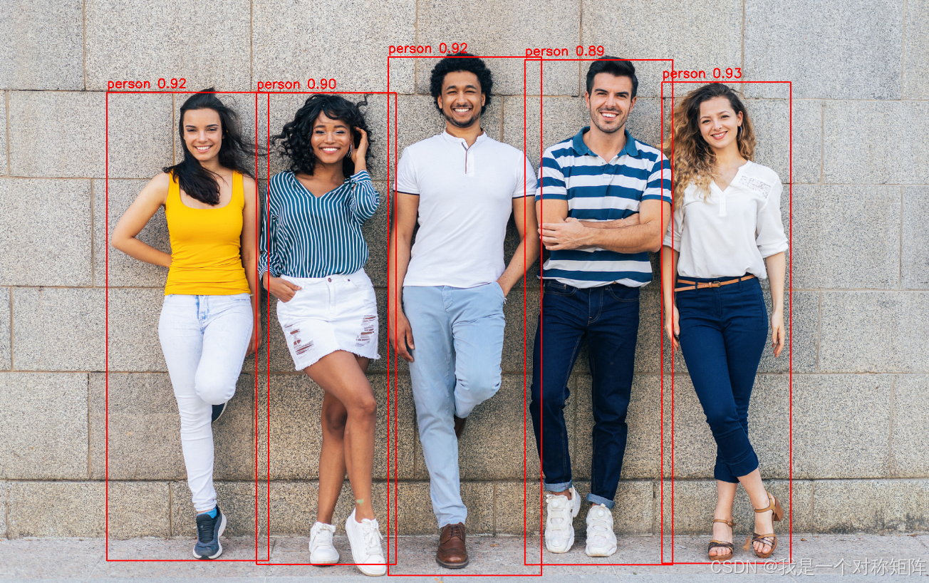
代码大体流程为:创建onnx推理session-->图像预处理-->onnx推理-->后处理(过滤bbox、非极大值抑制处理)-->可视化。上面的代码中大部分都是后处理。
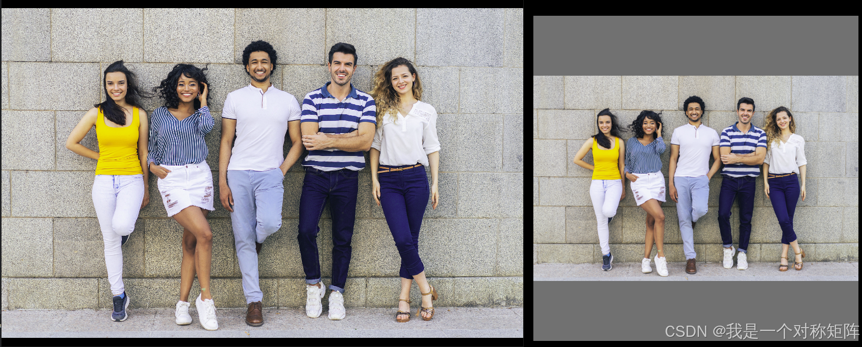
预处理中使用letterbox缩放扩充到(640,640),然后像素范围缩放到0~1,再reshape为(1,3,640,640)。
我们通过netron可视化onnx模型看到,yolov5s有三个尺度输出,最终得到25200个bbox。所以大部分的bbox都是得分极低的背景,我们需要对输出进行筛选。
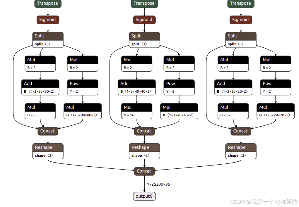
在filter_detections_onnx筛选函数中可以看到,模型的直接输出shape=(1,25200,85),每个框用85个数据表示,具体含义为=(cx,cy,w,h,bbox_score,clas1_score,clas2_score,…,clas80_score),即4个框的位置信息,1个框置信度,和80个类别的得分概率。
首先需要重新计算每个框的得分,一个框有两个属性:框位置得分,最大类别得分,那么最终得分就是=bbox_score*max_clas_score,所以后80个数值中最大值和bbox_score乘积就是最终得分,再加上最大类别序号,新的bbox=(cx,cy,w,h,bbox_scoremax_clas_score,clas_id)。然后将bbox_scoremax_clas_score低于阈值(比如0.5)的过滤掉,就得到结果(1,49,6),即49个框。
图中有5个框,现在有49个框,是因为有框重叠,需要进行非极大值抑制。不懂的朋友可以看看:非最大抑制。经过nms函数处理后,就得到(1,5,6)。
最后进行坐标转换,这里有多种转换。
首先是模型接收的是下右图的letterbox图像,所以输出的坐标是相对于右图的。我们需要将其转换到左图(即原图)去。
二是将(cx,cy,w,h)转为(x1,y1,x2,y2),当然这不是必须的,看需求而定。
3、TensoRT环境搭建
参考《cap2:1000分类的ResNet的TensorRT部署指南(python版)》中的3、环境搭建部分。
4、TensorRT序列化
这一节是将ONNX模型转换为TensorRT模型,即序列化的过程。该过程请完全参考参考《cap2:1000分类的ResNet的TensorRT部署指南(python版)》中的4、转换TensorRT引擎部分。
实际上可以看到模型的序列化和是哪种任务模型没有关系,无论哪种模型都是由基本算子如卷积、池化、BN等构成,在序列化时会将这些算子依此转换优化。只要不是一些特殊的奇葩的算子,都可以成功转换。当然如果是一些特殊的奇葩的,TensorRT暂时不支持的,TensorRT也提供了自己写算子的方法,这样任何模型都可以进行转换部署了。
5、推理
5.1 完整代码
推理代码也十分简单,先给出全部代码:
import time

import tensorrt as trt
import pycuda.driver as cuda
import pycuda.autoinit  # cuda初始化

import cv2
import numpy as np

TRT_LOGGER = trt.Logger(trt.Logger.WARNING)


def get_coco_label(class_id):
    """
    根据 COCO 数据集的 class_id 返回对应的类别名称。

    参数:
    - class_id: int,类别索引 (0-79)

    返回:
    - str,类别名称,如果 ID 超出范围,则返回 "Unknown"
    """
    coco_labels = [
        "person", "bicycle", "car", "motorcycle", "airplane", "bus", "train", "truck", "boat", "traffic light",
        "fire hydrant", "stop sign", "parking meter", "bench", "bird", "cat", "dog", "horse", "sheep", "cow",
        "elephant", "bear", "zebra", "giraffe", "backpack", "umbrella", "handbag", "tie", "suitcase", "frisbee",
        "skis", "snowboard", "sports ball", "kite", "baseball bat", "baseball glove", "skateboard", "surfboard",
        "tennis racket", "bottle", "wine glass", "cup", "fork", "knife", "spoon", "bowl", "banana", "apple",
        "sandwich", "orange", "broccoli", "carrot", "hot dog", "pizza", "donut", "cake", "chair", "couch",
        "potted plant", "bed", "dining table", "toilet", "TV", "laptop", "mouse", "remote", "keyboard",
        "cell phone", "microwave", "oven", "toaster", "sink", "refrigerator", "book", "clock", "vase",
        "scissors", "teddy bear", "hair drier", "toothbrush"
    ]

    if 0 <= class_id < len(coco_labels):
        return coco_labels[class_id]
    else:
        return "Unknown"

def load_engine(engine_file_path):
    """
    从engine模型反序列化
    :param engine_file_path:
    :return:
    """
    """加载 TensorRT 引擎"""
    with open(engine_file_path, "rb") as f, trt.Runtime(TRT_LOGGER) as runtime:
        return runtime.deserialize_cuda_engine(f.read())


def allocate_buffers(engine):
    """
    给模型直接输入和输出分配CUDA缓存区
    :param engine:
    :return:
    """
    inputs, outputs, bindings = [], [], []
    stream = cuda.Stream()

    for binding in engine:  # 遍历模型engine中的所有输入输出节点

        size = trt.volume(engine.get_tensor_shape(binding)) * np.dtype(np.float32).itemsize
        device_mem = cuda.mem_alloc(size)  # 分配size大小的空间,用于储存该节点的数据
        engine.get_tensor_mode(binding)
        if engine.get_tensor_mode(binding) == trt.TensorIOMode.INPUT:
            inputs.append(device_mem)  # 如果是输入节点则将该空间地址存入inputs
        elif engine.get_tensor_mode(binding) == trt.TensorIOMode.OUTPUT:
            outputs.append(device_mem)  # 如果是输出节点则将该空间地址存入outputs

        bindings.append(int(device_mem))

    return inputs, outputs, bindings, stream


class YoloTRT:
    def __init__(self, engine):
        self.context = engine.create_execution_context()  # 创建推理的上下文环境
        self.inputs, self.outputs, self.bindings, self.stream = allocate_buffers(engine)  # 初始化分配CUDA显存空间
        self.letter_process_meta = {}

    def letterbox(self, img_path, dst_size):
        image = cv2.imread(img_path)
        # 获取图像的原始尺寸
        height, width, channel = image.shape

        # 确定最长边
        max_side = max(height, width)

        # 计算缩放比例
        scale = dst_size / max_side

        # 计算缩放后的尺寸
        new_width = int(width * scale)
        new_height = int(height * scale)

        # 缩放图像
        resized_image = cv2.resize(image, (new_width, new_height), interpolation=cv2.INTER_AREA)

        # 创建一个64x64的黑色背景图像
        final_image = np.full((dst_size, dst_size, 3), 114, dtype=np.uint8)

        # 计算填充位置
        x_offset = (dst_size - new_width) // 2
        y_offset = (dst_size - new_height) // 2

        # 将缩放后的图像放入中心位置
        final_image[y_offset:y_offset + new_height, x_offset:x_offset + new_width] = resized_image

        # 记录预处理时的信息,方便后处理时坐标转换
        self.letter_process_meta['src_height'] = height
        self.letter_process_meta['src_width'] = width
        self.letter_process_meta['scale'] = scale
        self.letter_process_meta['x_offset'] = x_offset
        self.letter_process_meta['y_offset'] = y_offset

        return final_image

    def preprocess(self, img_path, input_shape):
        letter_image = self.letterbox(img_path, input_shape)
        input_data = letter_image / 255.0  # 归一化
        input_data = input_data.transpose(2, 0, 1)  # 转换维度顺序为 (C, H, W)
        input_data = np.expand_dims(input_data, axis=0)  # 添加 batch 维度
        input_data = input_data.astype(np.float32)  # 转换为 float32
        input_data=np.ascontiguousarray(input_data)
        return input_data

    def infer(self, image):
        # 将输入数据拷贝到 GPU
        cuda.memcpy_htod_async(self.inputs[0], image, self.stream)  # image是cpu的ram数据,需要拷贝到GPU,才能被tensorrt推理使用
        # 执行推理
        self.context.execute_async_v2(self.bindings, self.stream.handle, None)  # 推理
        # 从 GPU 拷贝输出结果
        # 初始化一个cpu的ram空间,方便从gpu接受输出数据,数据量为25200*85
        output = np.empty((1, 25200, 85), dtype=np.float32)
        cuda.memcpy_dtoh_async(output, self.outputs[0], self.stream)  # 将位于gpu上的输出数据复制到cpu上,方便对齐操作
        self.stream.synchronize()  # 同步,gpu是并行的,这里相当于等待同步一下

        return output  # 最后将输出结果返回

    def filter_detections_onnx(self, outputs, conf_threshold=0.25):
        """
        模型的直接输出shape=(1,25200,85),每个框用85个数据表示,具体含义为=(cx,cy,w,h,bbox_score,clas1_score,clas2_score,...,clas80_score)
        这一步要去除得分低于0.25的bbox框,去除低置信度目标,返回 shape (1, N, 6),每个框用6个数据表示,具体含义为=(cx,cy,w,h,bbox_score*max_clas_score,clas_id)

        参数:
        - onnx_output: 模型的输出,形状为 (1, 25200, 85)
        - conf_threshold: 置信度阈值,默认 0.25

        返回:
        - filtered_output: 经过筛选后的张量,形状为 (1, N, 6),N 为保留目标数量
                          每个目标包含 (x, y, w, h, score, class_id)
        """
        # 取出 batch 维度
        predictions = outputs[0]  # (25200, 85)

        # 提取 (x, y, w, h)
        bboxes = predictions[:, :4]  # (25200, 4)

        # 提取目标置信度
        objectness = predictions[:, 4]  # (25200,)

        # 计算类别置信度 scores = objectness * class_probs
        class_probs = predictions[:, 5:]  # (25200, 80)
        class_scores = np.max(class_probs, axis=1)  # 取最大类别得分 (25200,)
        class_ids = np.argmax(class_probs, axis=1)  # 取类别索引 (25200,)

        # 计算最终得分
        scores = objectness * class_scores  # (25200,)

        # 过滤低置信度目标
        mask = scores > conf_threshold
        filtered_bboxes = bboxes[mask]  # (N, 4)
        filtered_scores = scores[mask]  # (N,)
        filtered_class_ids = class_ids[mask]  # (N,)

        # 组合结果 (N, 6)
        filtered_output = np.column_stack((filtered_bboxes, filtered_scores, filtered_class_ids))

        # 添加 batch 维度,最终 shape 为 (1, N, 6)
        return np.expand_dims(filtered_output, axis=0)  # (1, N, 6)

    def compute_iou(self, box, boxes):
        """
        计算一个框与多个框的 IOU (交并比)

        参数:
        - box: (x, y, w, h) 单个框
        - boxes: (N, 4) 其他框

        返回:
        - ious: (N,) 的 IOU 数组
        """
        x, y, w, h = box
        x1, y1, x2, y2 = x - w / 2, y - h / 2, x + w / 2, y + h / 2

        x_boxes, y_boxes, w_boxes, h_boxes = boxes.T
        x1_boxes, y1_boxes, x2_boxes, y2_boxes = x_boxes - w_boxes / 2, y_boxes - h_boxes / 2, x_boxes + w_boxes / 2, y_boxes + h_boxes / 2

        inter_x1 = np.maximum(x1, x1_boxes)
        inter_y1 = np.maximum(y1, y1_boxes)
        inter_x2 = np.minimum(x2, x2_boxes)
        inter_y2 = np.minimum(y2, y2_boxes)

        inter_area = np.maximum(0, inter_x2 - inter_x1) * np.maximum(0, inter_y2 - inter_y1)
        box_area = w * h
        boxes_area = w_boxes * h_boxes

        union_area = box_area + boxes_area - inter_area
        ious = inter_area / (union_area + 1e-6)  # 避免除零

        return ious

    def nms(self, detections, iou_threshold=0.45):
        """
        对经过置信度过滤后的检测框进行非极大值抑制 (NMS)

        参数:
        - detections: 形状为 (1, N, 6) 的数组,其中每个目标包含 (x, y, w, h, score, class_id)
        - iou_threshold: IOU 阈值,默认 0.45

        返回:
        - nms_detections: 形状为 (1, M, 6) 的数组,M 为 NMS 后的目标数
        """
        if detections.shape[1] == 0:
            return detections  # 无目标则直接返回

        detections = detections[0]  # 去除 batch 维度,变成 (N, 6)

        # 按置信度降序排序
        indices = np.argsort(detections[:, 4])[::-1]
        detections = detections[indices]

        keep = []
        while len(detections) > 0:
            # 取出当前置信度最高的框
            best = detections[0]
            keep.append(best)

            if len(detections) == 1:
                break  # 只剩下一个框,直接退出

            # 计算当前框与剩余框的 IOU
            ious = self.compute_iou(best[:4], detections[1:, :4])

            # 过滤掉 IOU 大于阈值的框
            detections = detections[1:][ious < iou_threshold]

        # 转换回 (1, M, 6) 形状
        return np.expand_dims(np.array(keep), axis=0)

    def cxcywh_convert(self, outputs):
        H, W = self.letter_process_meta['src_height'], self.letter_process_meta['src_width']
        scale = self.letter_process_meta['scale']
        x_offset = self.letter_process_meta['x_offset']
        y_offset = self.letter_process_meta['y_offset']

        results = []
        for batch_bboxs in outputs:
            result = []
            for bbox in batch_bboxs:
                cx, cy, w, h, score, clas_id = bbox
                cx = (cx - x_offset) / (W * scale)
                cy = (cy - y_offset) / (H * scale)
                w = w / (W * scale)
                h = h / (H * scale)
                result.append([cx, cy, w, h,score, clas_id])
            results.append(result)
        return results

    def postprocess(self, outputs):
        outputs = self.filter_detections_onnx(outputs, 0.5)
        outputs = self.nms(outputs)
        outputs = self.cxcywh_convert(outputs)
        return outputs

    def visual(self,outputs,img_path):
        image=cv2.imread(img_path)
        H,W,C=image.shape

        for batch_bboxs in outputs:
            for bbox in batch_bboxs:
                cx, cy, w, h, score, clas_id = bbox

                # (cx,cy,w,h)-->(x1,y1,x2,y2)
                x1 = int((cx - w / 2) * W)
                y1 = int((cy - h / 2) * H)
                x2 = int((cx + w / 2) * W)
                y2 = int((cy + h / 2) * H)

                #
                cls = get_coco_label(int(clas_id))
                # visual
                cv2.rectangle(image, (x1, y1), (x2, y2), (0, 0, 255), 4)
                cv2.putText(image, f'{cls} {score:.2f}', (x1, y1 - 10), cv2.FONT_HERSHEY_SIMPLEX, 1.2, (0, 0, 255),
                            2)

        # 显示结果
        cv2.imshow('Result', image)
        cv2.waitKey(0)
        cv2.destroyAllWindows()


if __name__ == "__main__":
    engine_path = "yolov5s.engine"

    engine = load_engine(engine_path)

    yoloTrt = YoloTRT(engine)  # 初始化一次

    input_data = yoloTrt.preprocess("test.jpeg", 640)
    for i in range(10):
        t1=time.time()
        output = yoloTrt.infer(input_data)  # 推理
        print(time.time()-t1)

    output = yoloTrt.postprocess(output)    # 后处理

    yoloTrt.visual(output,"test.jpeg")      # 可视化
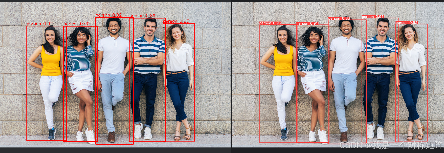
左图是TensorRT的结果,耗时0.002s(仅统计infer环节),右侧是Pytorch的Yolov5直接测试结果。
5.2 推理代码分析
上面的代码有318行,但是其中预处理yoloTrt.preprocess、后处理yoloTrt.postprocess和可视化yoloTrt.visual这几部分和TensorRT没有任何关系,完全是python的处理过程而已。除去这几部分就只剩下78行:
import tensorrt as trt
import pycuda.driver as cuda
import pycuda.autoinit  # cuda初始化

import numpy as np

TRT_LOGGER = trt.Logger(trt.Logger.WARNING)


def load_engine(engine_file_path):
    """
    从engine模型反序列化
    :param engine_file_path:
    :return:
    """
    """加载 TensorRT 引擎"""
    with open(engine_file_path, "rb") as f, trt.Runtime(TRT_LOGGER) as runtime:
        return runtime.deserialize_cuda_engine(f.read())


def allocate_buffers(engine):
    """
    给模型直接输入和输出分配CUDA缓存区
    :param engine:
    :return:
    """
    inputs, outputs, bindings = [], [], []
    stream = cuda.Stream()

    for binding in engine:  # 遍历模型engine中的所有输入输出节点

        size = trt.volume(engine.get_tensor_shape(binding)) * np.dtype(np.float32).itemsize
        device_mem = cuda.mem_alloc(size)  # 分配size大小的空间,用于储存该节点的数据
        engine.get_tensor_mode(binding)
        if engine.get_tensor_mode(binding) == trt.TensorIOMode.INPUT:
            inputs.append(device_mem)  # 如果是输入节点则将该空间地址存入inputs
        elif engine.get_tensor_mode(binding) == trt.TensorIOMode.OUTPUT:
            outputs.append(device_mem)  # 如果是输出节点则将该空间地址存入outputs

        bindings.append(int(device_mem))

    return inputs, outputs, bindings, stream


class YoloTRT:
    def __init__(self, engine):
        self.context = engine.create_execution_context()  # 创建推理的上下文环境
        self.inputs, self.outputs, self.bindings, self.stream = allocate_buffers(engine)  # 初始化分配CUDA显存空间


    def infer(self, image):
        # 将输入数据拷贝到 GPU
        cuda.memcpy_htod_async(self.inputs[0], image, self.stream)  # image是cpu的ram数据,需要拷贝到GPU,才能被tensorrt推理使用
        # 执行推理
        self.context.execute_async_v2(self.bindings, self.stream.handle, None)  # 推理
        # 从 GPU 拷贝输出结果
        # 初始化一个cpu的ram空间,方便从gpu接受输出数据,数据量为25200*85
        output = np.empty((1, 25200, 85), dtype=np.float32)
        cuda.memcpy_dtoh_async(output, self.outputs[0], self.stream)  # 将位于gpu上的输出数据复制到cpu上,方便对齐操作
        self.stream.synchronize()  # 同步,gpu是并行的,这里相当于等待同步一下

        return output  # 最后将输出结果返回


if __name__ == "__main__":
    engine_path = "yolov5s.engine"

    engine = load_engine(engine_path)

    yoloTrt = YoloTRT(engine)  # 初始化一次

    # input_data = yoloTrt.preprocess("test.jpeg", 640)     # 输入预处理

    output = yoloTrt.infer(input_data)  # 推理

    # output = yoloTrt.postprocess(output)    # 后处理
可以看到首先我们使用load_engine从engine文件反序列化模型,加载到RAM中。在YoloTRT的__init__构造函数中,我们创建了推理的上下文环境,完成了CUDA显存空间的分配。
为什么要分配显存空间,因为CUDA程序只能读取位于显存上的数据,而一般程序读取得数据都位于RAM。所以我们需要先在CUDA上用cuda.mem_alloc为模型推理的输入和输出开辟足够的空间,然后将python读取的图像数据用cuda.memcpy_htod_async复制到CUDA显存中去,推理时直接从显存读取数据。推理结束后,输出放在显存上,再使用cuda.memcpy_dtoh_async将结果从显存复制到RAM中。同理接收数据时,需要再RAM中开辟足够的空间接收从显存来的数据,所以使用output = np.empty((1, 25200, 85), dtype=np.float32)开辟了足够大小的空间。
在推理时就是将数据复制到显存,执行推理,将结果复制到RAM中,然后再使用python进行相应的后处理即可。
所以基于Python的TensorRT部署其实也非常简单,有着固定的流程。预处理和后处理都可以使用Python实现。需要TensorRT处理的代码只有短短十几行。