当前位置：首页 > news >正文

《Python星球日记》第53天：卷积神经网络（CNN）入门

news 来源：原创 2025/5/11 10:40:13

名人说：路漫漫其修远兮，吾将上下而求索。—— 屈原《离骚》
创作者：Code_流苏(CSDN)（一个喜欢古诗词和编程的Coder😊）

目录

一、图像表示与通道概念
1. 数字图像的本质
2. RGB颜色模型
3. 图像预处理

二、卷积神经网络的基本组件
1. 卷积层（Convolutional Layer）
2. 池化层（Pooling Layer）
3. 全连接层（Fully Connected Layer）

三、CNN的优势与应用场景
1. CNN的核心优势
2. 主要应用场景

四、使用TensorFlow实现简单CNN
1. 环境准备与数据加载
2. 构建CNN模型
3. 训练模型
4. 评估模型

五、PyTorch版本实现
六、实战练习：MNIST手写数字识别
1. 完整代码实现
2. 代码解析
3. 运行结果分析

七、总结与进阶
1. 关键知识点回顾
2. 进阶方向
3. 推荐资源

八、实战练习

👋 专栏介绍： Python星球日记专栏介绍（持续更新ing）
✅ 上一篇：《Python星球日记》第52天：反向传播与优化器

欢迎来到Python星球的第53天！🪐

今天我们将探索深度学习中最重要的架构之一——卷积神经网络（CNN）。CNN在计算机视觉领域取得了革命性的突破，让机器能够"看懂"图像。

无论你是想开发图像识别应用、自动驾驶系统，还是医疗诊断工具，CNN都是必不可少的基础知识。让我们一起踏上这段激动人心的旅程吧！

一、图像表示与通道概念

1. 数字图像的本质

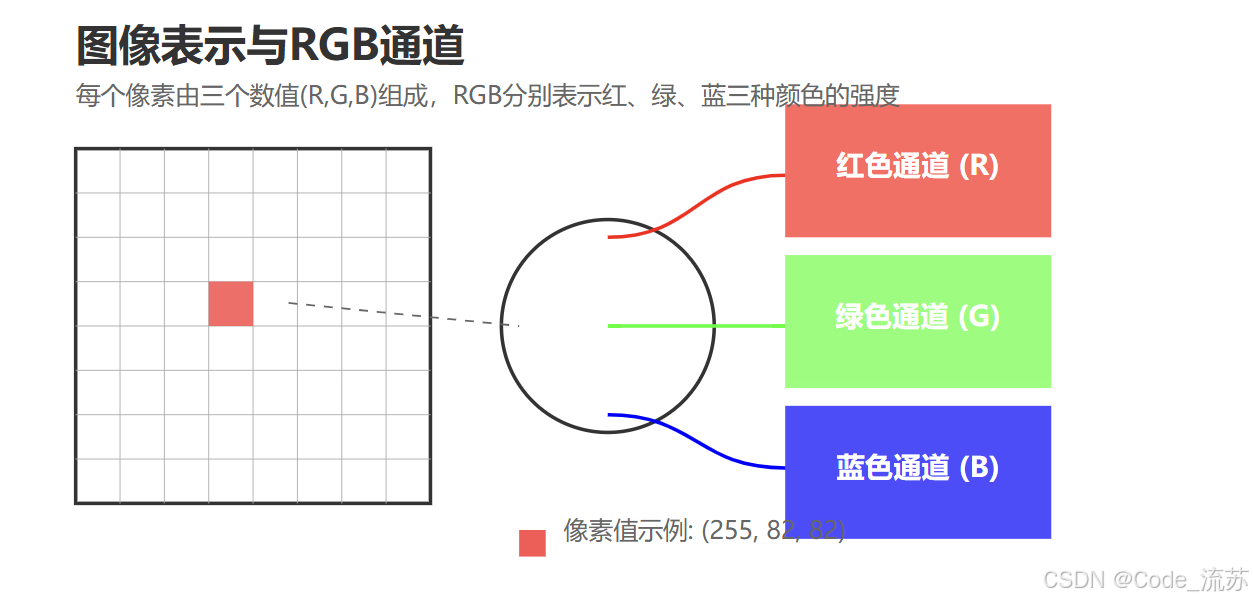
在计算机的世界里，图像本质上是多维数组。当我们看到一张彩色照片时，计算机看到的是一个三维数组：

高度（Height）：图像的垂直像素数
宽度（Width）：图像的水平像素数
通道（Channels）：描述每个像素的颜色信息

2. RGB颜色模型

最常见的彩色图像使用RGB颜色模型：

R通道：表示红色（Red）的强度，数值范围为0-255
G通道：表示绿色（Green）的强度，数值范围为0-255
B通道：表示蓝色（Blue）的强度，数值范围为0-255

对于灰度图像，我们只需要一个通道，数值表示像素的亮度（0为黑色，255为白色）。

在这里插入图片描述

3. 图像预处理

在将图像输入CNN之前，通常需要进行标准化处理，将像素值缩放到0-1范围内（除以255）。这样做有助于网络更快地收敛，提高训练效率。

# 图像预处理示例
import numpy as np
from PIL import Image# 读取图像
img = Image.open('example.jpg')
img_array = np.array(img)# 标准化处理
normalized_img = img_array / 255.0

二、卷积神经网络的基本组件

CNN的强大之处在于其特殊的网络架构，主要由以下组件构成：

在这里插入图片描述

1. 卷积层（Convolutional Layer）

卷积层是CNN的核心组件，负责提取图像的特征。卷积操作通过一个小的卷积核（也称为滤波器或权重矩阵）在输入图像上滑动，计算卷积核与图像局部区域的点积，从而生成特征图（Feature Map）。

在这里插入图片描述

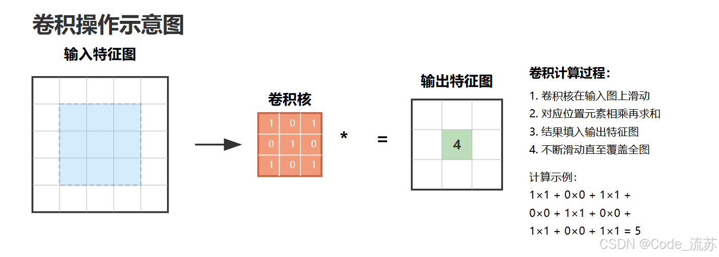
卷积层的几个重要概念：

卷积核大小：通常为3×3或5×5的小矩阵，决定了感受野的大小
步长（Stride）：卷积核在图像上移动的步长，控制特征图的大小
填充（Padding）：在输入图像周围添加像素（通常为0），以保持特征图尺寸
激活函数：通常使用ReLU激活函数，将负值置为0，引入非线性

# TensorFlow中定义卷积层
import tensorflow as tf# 创建一个2D卷积层，使用32个3x3的卷积核
conv_layer = tf.keras.layers.Conv2D(filters=32,           # 卷积核数量kernel_size=(3, 3),   # 卷积核大小strides=(1, 1),       # 步长padding='same',       # 填充方式，'same'保持输出尺寸与输入相同activation='relu'     # 激活函数
)

2. 池化层（Pooling Layer）

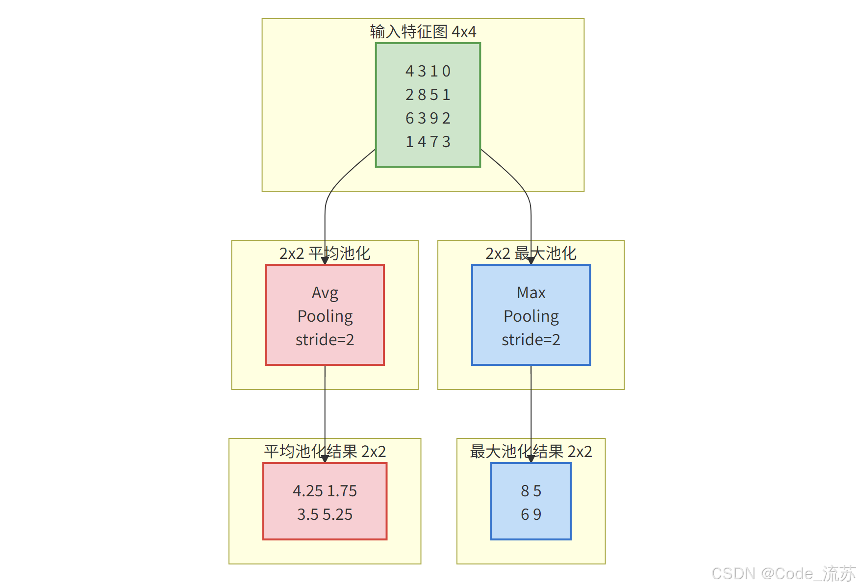
池化层的主要作用是降维，减少参数数量和计算负担，同时提高模型对图像位置变化的鲁棒性。

常见的池化操作有：

最大池化（Max Pooling）：取区域内的最大值
平均池化（Average Pooling）：取区域内的平均值

在这里插入图片描述

# TensorFlow中定义池化层
max_pool = tf.keras.layers.MaxPool2D(pool_size=(2, 2),     # 池化窗口大小strides=(2, 2),       # 步长padding='valid'       # 不使用填充
)

3. 全连接层（Fully Connected Layer）

在CNN的末端，通常会使用全连接层将提取到的特征映射到最终的输出类别。全连接层与传统神经网络中的隐藏层相同，每个神经元与前一层的所有神经元相连。

# 在CNN中添加全连接层
model = tf.keras.Sequential([# ... 卷积层和池化层 ...# 将特征图展平为一维向量tf.keras.layers.Flatten(),# 全连接层tf.keras.layers.Dense(128, activation='relu'),tf.keras.layers.Dense(10, activation='softmax')  # 10分类问题
])

三、CNN的优势与应用场景

1. CNN的核心优势

相比传统神经网络，卷积神经网络具有以下显著优势：

参数共享：同一个卷积核在整个图像上滑动，大大减少了参数数量
局部连接：每个神经元只与输入数据的一个局部区域相连，捕捉局部特征
平移不变性：无论特征在图像中的位置如何变化，CNN都能够识别出来
层次化特征学习：浅层网络学习简单特征（如边缘、纹理），深层网络学习更复杂的特征（如目标的部分或整体）

2. 主要应用场景

CNN在计算机视觉领域有广泛应用：

图像分类：识别图像中的主要对象（如ImageNet挑战赛）
目标检测：定位并识别图像中的多个对象（如YOLO、Faster R-CNN）
图像分割：为图像中的每个像素分配类别（如U-Net）
人脸识别：识别和验证人脸身份
医学影像分析：识别X光、CT、MRI等医学图像中的异常
自动驾驶：感知和理解道路环境

四、使用TensorFlow实现简单CNN

下面我们将使用TensorFlow框架实现一个简单的CNN模型，用于手写数字识别。

1. 环境准备与数据加载

# 导入必要的库
import tensorflow as tf
import numpy as np
import matplotlib.pyplot as plt# 加载MNIST数据集
(x_train, y_train), (x_test, y_test) = tf.keras.datasets.mnist.load_data()# 数据预处理
x_train = x_train.reshape(-1, 28, 28, 1).astype('float32') / 255.0
x_test = x_test.reshape(-1, 28, 28, 1).astype('float32') / 255.0# 将标签转换为one-hot编码
y_train = tf.keras.utils.to_categorical(y_train, 10)
y_test = tf.keras.utils.to_categorical(y_test, 10)print("训练集形状:", x_train.shape)
print("测试集形状:", x_test.shape)

在这里插入图片描述

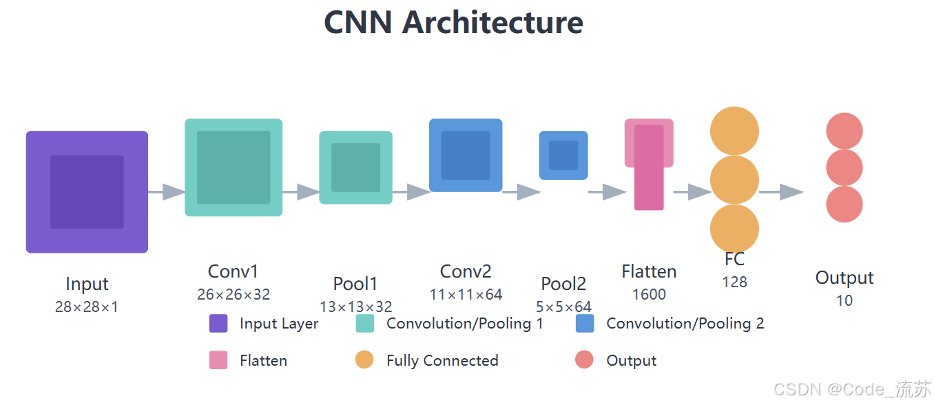
2. 构建CNN模型

# 定义一个简单的CNN模型
def create_mnist_cnn():model = tf.keras.Sequential([# 第一个卷积块tf.keras.layers.Conv2D(32, (3, 3), activation='relu', padding='same', input_shape=(28, 28, 1)),tf.keras.layers.MaxPooling2D((2, 2)),# 第二个卷积块tf.keras.layers.Conv2D(64, (3, 3), activation='relu', padding='same'),tf.keras.layers.MaxPooling2D((2, 2)),# 展平层tf.keras.layers.Flatten(),# 全连接层tf.keras.layers.Dense(128, activation='relu'),tf.keras.layers.Dropout(0.5),  # 防止过拟合tf.keras.layers.Dense(10, activation='softmax')  # 10个数字类别])return model# 创建模型
model = create_mnist_cnn()# 编译模型
model.compile(optimizer='adam',loss='categorical_crossentropy',metrics=['accuracy']
)# 查看模型结构
model.summary()

在这里插入图片描述

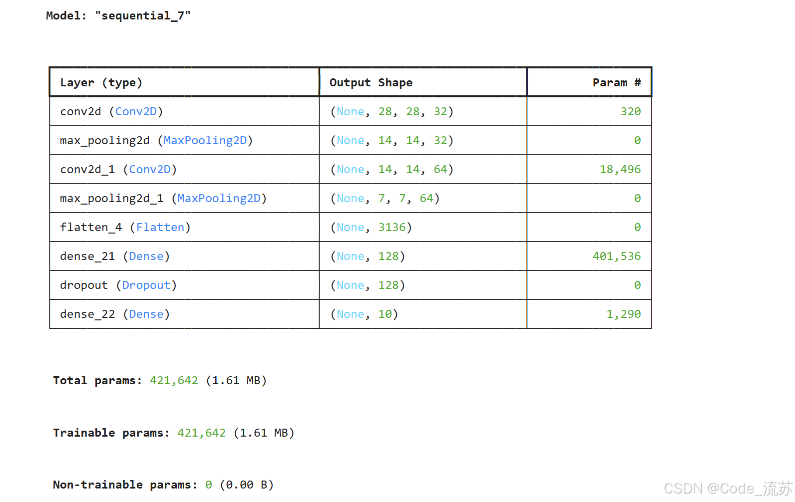
上面的模型包含两个卷积块，每个卷积块包含一个卷积层和一个池化层。模型的最后是全连接层，用于将提取的特征映射到10个数字类别。注意我们添加了Dropout层来防止过拟合。

3. 训练模型

# 训练模型
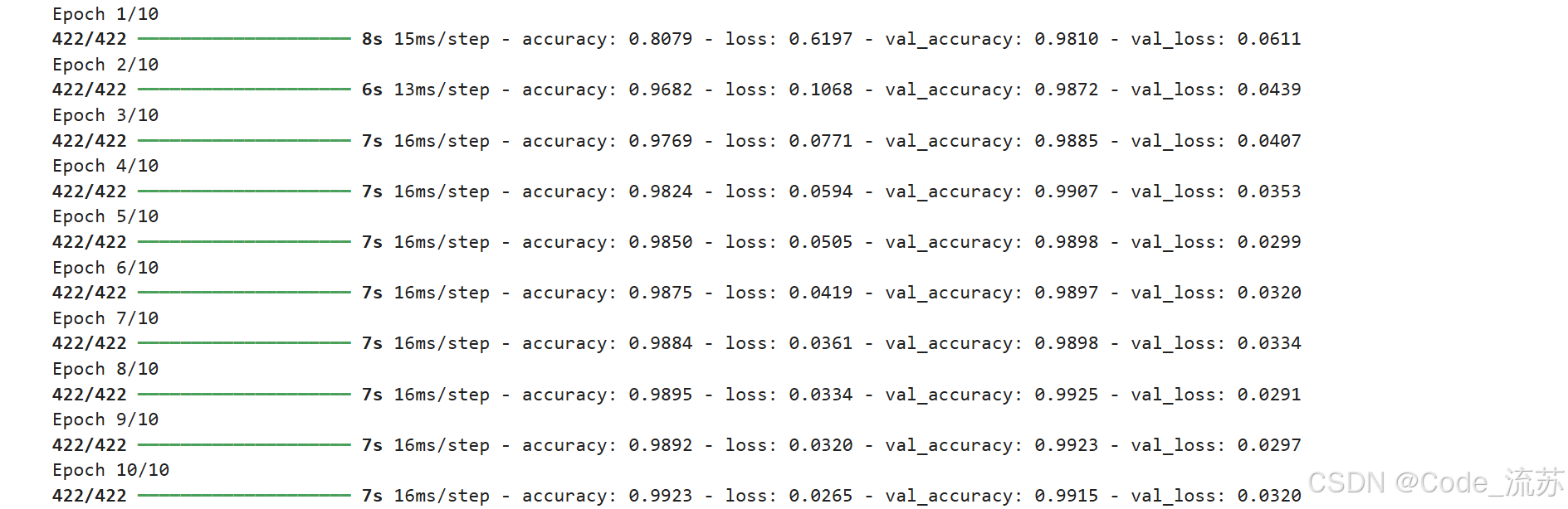
history = model.fit(x_train, y_train,epochs=10,batch_size=128,validation_split=0.1,verbose=1
)# 绘制训练历史
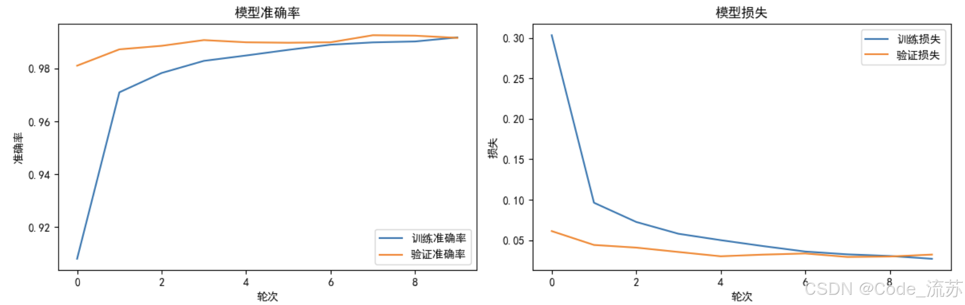
plt.figure(figsize=(12, 4))# 准确率变化
plt.subplot(1, 2, 1)
plt.plot(history.history['accuracy'], label='训练准确率')
plt.plot(history.history['val_accuracy'], label='验证准确率')
plt.title('模型准确率')
plt.xlabel('轮次')
plt.ylabel('准确率')
plt.legend()# 损失变化
plt.subplot(1, 2, 2)
plt.plot(history.history['loss'], label='训练损失')
plt.plot(history.history['val_loss'], label='验证损失')
plt.title('模型损失')
plt.xlabel('轮次')
plt.ylabel('损失')
plt.legend()plt.tight_layout()
plt.show()

在这里插入图片描述

4. 评估模型

# 在测试集上评估模型
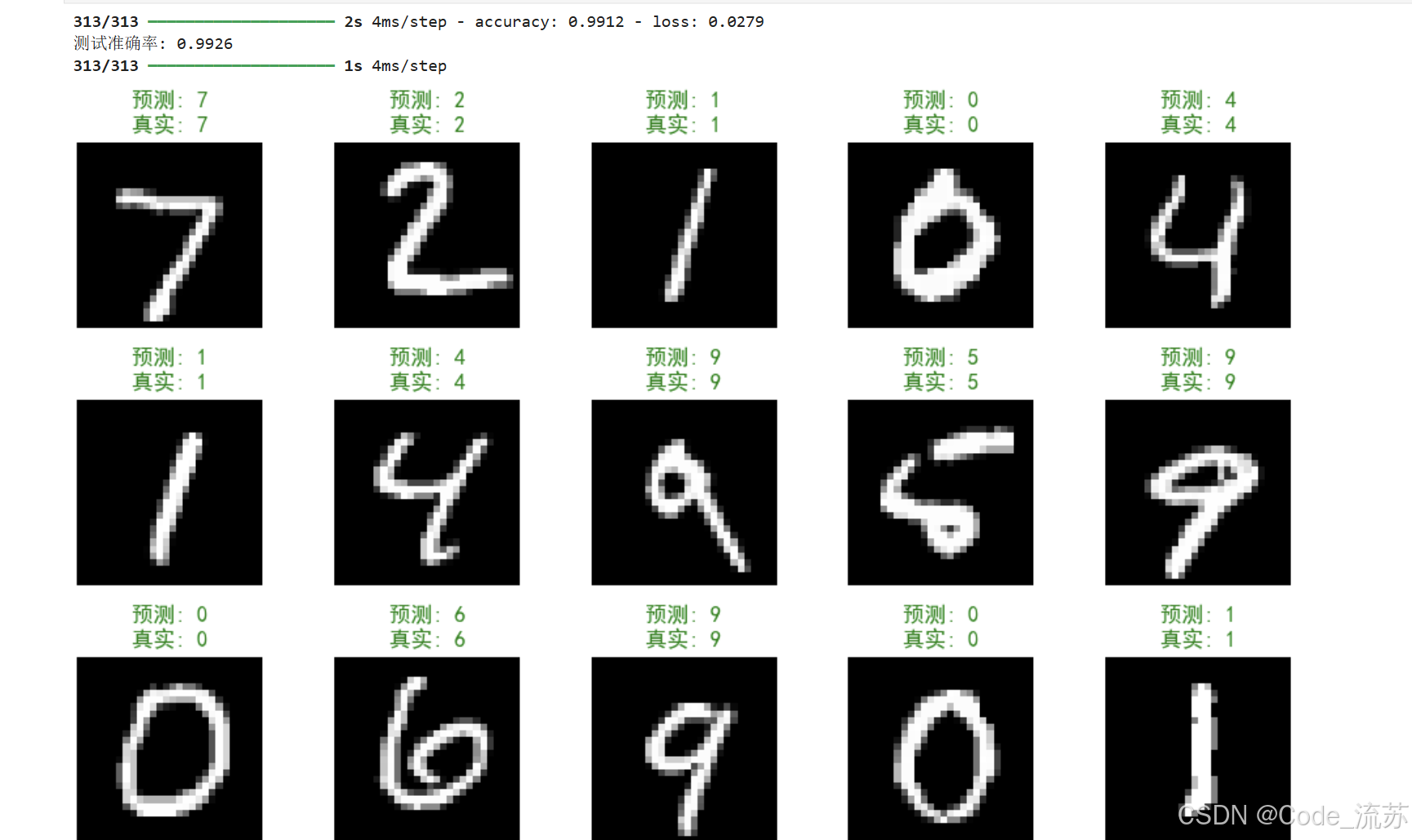
test_loss, test_acc = model.evaluate(x_test, y_test)
print(f"测试准确率: {test_acc:.4f}")# 进行预测
predictions = model.predict(x_test)
predicted_classes = np.argmax(predictions, axis=1)
true_classes = np.argmax(y_test, axis=1)# 显示一些预测结果
plt.figure(figsize=(10, 10))
for i in range(25):plt.subplot(5, 5, i+1)plt.imshow(x_test[i].reshape(28, 28), cmap='gray')prediction = predicted_classes[i]true_label = true_classes[i]color = 'green' if prediction == true_label else 'red'plt.title(f"预测: {prediction}\n真实: {true_label}", color=color)plt.axis('off')plt.tight_layout()
plt.show()

在这里插入图片描述

五、PyTorch版本实现

如果你更喜欢使用PyTorch框架，下面是等效的实现：

# 导入必要的库
import torch
import torch.nn as nn
import torch.optim as optim
import torchvision
import torchvision.transforms as transforms
import matplotlib.pyplot as plt
import numpy as np# 定义数据转换
transform = transforms.Compose([transforms.ToTensor(),transforms.Normalize((0.1307,), (0.3081,))  # MNIST数据集的均值和标准差
])# 加载MNIST数据集
train_dataset = torchvision.datasets.MNIST(root='./data', train=True, download=True, transform=transform)
test_dataset = torchvision.datasets.MNIST(root='./data', train=False, download=True, transform=transform)train_loader = torch.utils.data.DataLoader(train_dataset, batch_size=128, shuffle=True)
test_loader = torch.utils.data.DataLoader(test_dataset, batch_size=128, shuffle=False)# 定义CNN模型
class MnistCNN(nn.Module):def __init__(self):super(MnistCNN, self).__init__()# 第一个卷积块self.conv1 = nn.Conv2d(1, 32, kernel_size=3, padding=1)self.relu1 = nn.ReLU()self.pool1 = nn.MaxPool2d(kernel_size=2)# 第二个卷积块self.conv2 = nn.Conv2d(32, 64, kernel_size=3, padding=1)self.relu2 = nn.ReLU()self.pool2 = nn.MaxPool2d(kernel_size=2)# 全连接层self.flatten = nn.Flatten()self.fc1 = nn.Linear(64 * 7 * 7, 128)self.relu3 = nn.ReLU()self.dropout = nn.Dropout(0.5)self.fc2 = nn.Linear(128, 10)def forward(self, x):# 第一个卷积块x = self.conv1(x)x = self.relu1(x)x = self.pool1(x)# 第二个卷积块x = self.conv2(x)x = self.relu2(x)x = self.pool2(x)# 全连接层x = self.flatten(x)x = self.fc1(x)x = self.relu3(x)x = self.dropout(x)x = self.fc2(x)return x# 创建模型实例
device = torch.device("cuda" if torch.cuda.is_available() else "cpu")
model = MnistCNN().to(device)# 定义损失函数和优化器
criterion = nn.CrossEntropyLoss()
optimizer = optim.Adam(model.parameters(), lr=0.001)# 训练模型
num_epochs = 10
train_losses = []
train_accs = []
test_losses = []
test_accs = []for epoch in range(num_epochs):# 训练模式model.train()running_loss = 0.0correct = 0total = 0for images, labels in train_loader:images, labels = images.to(device), labels.to(device)# 前向传播outputs = model(images)loss = criterion(outputs, labels)# 反向传播和优化optimizer.zero_grad()loss.backward()optimizer.step()# 统计running_loss += loss.item() * images.size(0)_, predicted = torch.max(outputs.data, 1)total += labels.size(0)correct += (predicted == labels).sum().item()epoch_loss = running_loss / len(train_dataset)epoch_acc = correct / totaltrain_losses.append(epoch_loss)train_accs.append(epoch_acc)# 评估模式model.eval()test_loss = 0.0correct = 0total = 0with torch.no_grad():for images, labels in test_loader:images, labels = images.to(device), labels.to(device)outputs = model(images)loss = criterion(outputs, labels)test_loss += loss.item() * images.size(0)_, predicted = torch.max(outputs.data, 1)total += labels.size(0)correct += (predicted == labels).sum().item()test_loss = test_loss / len(test_dataset)test_acc = correct / totaltest_losses.append(test_loss)test_accs.append(test_acc)print(f"Epoch {epoch+1}/{num_epochs}, 训练损失: {epoch_loss:.4f}, 训练准确率: {epoch_acc:.4f}, 测试损失: {test_loss:.4f}, 测试准确率: {test_acc:.4f}")# 绘制训练历史
plt.figure(figsize=(12, 4))# 准确率变化
plt.subplot(1, 2, 1)
plt.plot(train_accs, label='训练准确率')
plt.plot(test_accs, label='测试准确率')
plt.title('模型准确率')
plt.xlabel('轮次')
plt.ylabel('准确率')
plt.legend()# 损失变化
plt.subplot(1, 2, 2)
plt.plot(train_losses, label='训练损失')
plt.plot(test_losses, label='测试损失')
plt.title('模型损失')
plt.xlabel('轮次')
plt.ylabel('损失')
plt.legend()plt.tight_layout()
plt.show()

六、实战练习：MNIST手写数字识别

现在让我们完整地实现一个手写数字识别系统，包括数据加载、模型定义、训练、评估和可视化。我将使用TensorFlow来实现这个项目。

1. 完整代码实现

import tensorflow as tf
import numpy as np
import matplotlib.pyplot as plt
from sklearn.metrics import confusion_matrix, classification_report
import seaborn as sns# 设置随机种子，确保结果可重现
np.random.seed(42)
tf.random.set_seed(42)# 1. 加载并预处理MNIST数据集
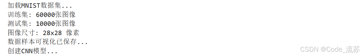
print("加载MNIST数据集...")
(x_train, y_train), (x_test, y_test) = tf.keras.datasets.mnist.load_data()# 查看数据集大小
print(f"训练集: {x_train.shape[0]}张图像")
print(f"测试集: {x_test.shape[0]}张图像")
print(f"图像尺寸: {x_train.shape[1]}x{x_train.shape[2]} 像素")# 数据预处理
x_train = x_train.reshape(-1, 28, 28, 1).astype('float32') / 255.0
x_test = x_test.reshape(-1, 28, 28, 1).astype('float32') / 255.0# 将标签转换为one-hot编码
y_train_onehot = tf.keras.utils.to_categorical(y_train, 10)
y_test_onehot = tf.keras.utils.to_categorical(y_test, 10)# 2. 可视化一些训练样本
plt.figure(figsize=(10, 5))
for i in range(10):plt.subplot(2, 5, i+1)plt.imshow(x_train[i].reshape(28, 28), cmap='gray')plt.title(f"标签: {y_train[i]}")plt.axis('off')
plt.tight_layout()
plt.savefig('mnist_samples.png')
plt.close()
print("数据样本可视化已保存...")# 3. 定义CNN模型
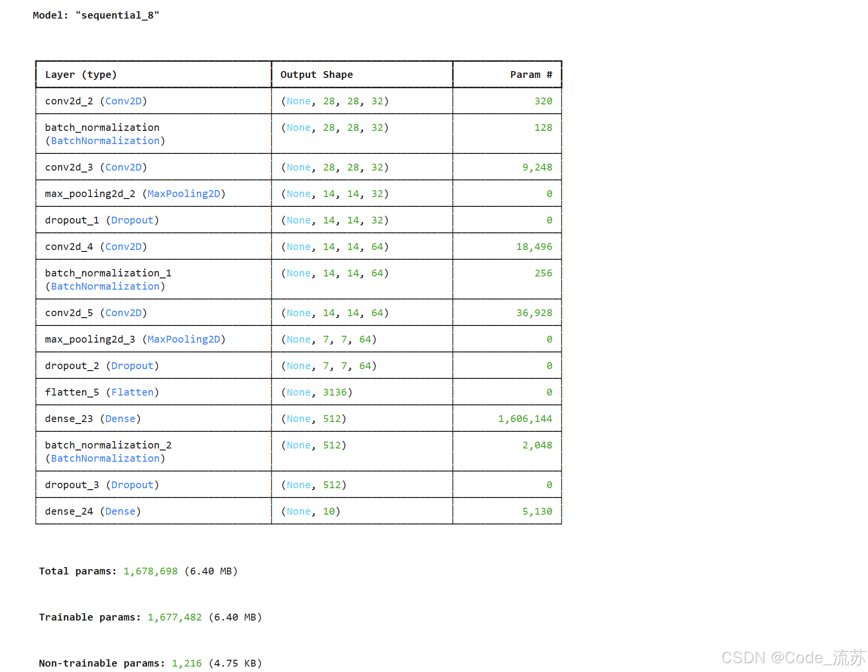
def create_cnn_model():model = tf.keras.Sequential([# 输入层tf.keras.layers.InputLayer(input_shape=(28, 28, 1)),# 第一个卷积块tf.keras.layers.Conv2D(32, (3, 3), padding='same', activation='relu'),tf.keras.layers.BatchNormalization(),tf.keras.layers.Conv2D(32, (3, 3), padding='same', activation='relu'),tf.keras.layers.MaxPooling2D((2, 2)),tf.keras.layers.Dropout(0.25),# 第二个卷积块tf.keras.layers.Conv2D(64, (3, 3), padding='same', activation='relu'),tf.keras.layers.BatchNormalization(),tf.keras.layers.Conv2D(64, (3, 3), padding='same', activation='relu'),tf.keras.layers.MaxPooling2D((2, 2)),tf.keras.layers.Dropout(0.25),# 展平层tf.keras.layers.Flatten(),# 全连接层tf.keras.layers.Dense(512, activation='relu'),tf.keras.layers.BatchNormalization(),tf.keras.layers.Dropout(0.5),tf.keras.layers.Dense(10, activation='softmax')])return model# 创建模型
print("创建CNN模型...")
model = create_cnn_model()
model.summary()# 编译模型
model.compile(optimizer=tf.keras.optimizers.Adam(learning_rate=0.001),loss='categorical_crossentropy',metrics=['accuracy']
)# 4. 定义回调函数
# 早停：如果验证损失在3个epoch内没有改善，则停止训练
early_stopping = tf.keras.callbacks.EarlyStopping(monitor='val_loss',patience=3,restore_best_weights=True
)# 学习率降低：如果验证损失在2个epoch内没有改善，则降低学习率
reduce_lr = tf.keras.callbacks.ReduceLROnPlateau(monitor='val_loss',factor=0.5,patience=2,min_lr=0.00001
)# 5. 训练模型
print("开始训练模型...")
history = model.fit(x_train, y_train_onehot,epochs=15,batch_size=128,validation_split=0.1,callbacks=[early_stopping, reduce_lr],verbose=1
)# 6. 绘制训练历史
plt.figure(figsize=(12, 4))# 准确率变化
plt.subplot(1, 2, 1)
plt.plot(history.history['accuracy'], label='训练准确率')
plt.plot(history.history['val_accuracy'], label='验证准确率')
plt.title('模型准确率')
plt.xlabel('轮次')
plt.ylabel('准确率')
plt.legend()# 损失变化
plt.subplot(1, 2, 2)
plt.plot(history.history['loss'], label='训练损失')
plt.plot(history.history['val_loss'], label='验证损失')
plt.title('模型损失')
plt.xlabel('轮次')
plt.ylabel('损失')
plt.legend()plt.tight_layout()
plt.savefig('training_history.png')
plt.close()
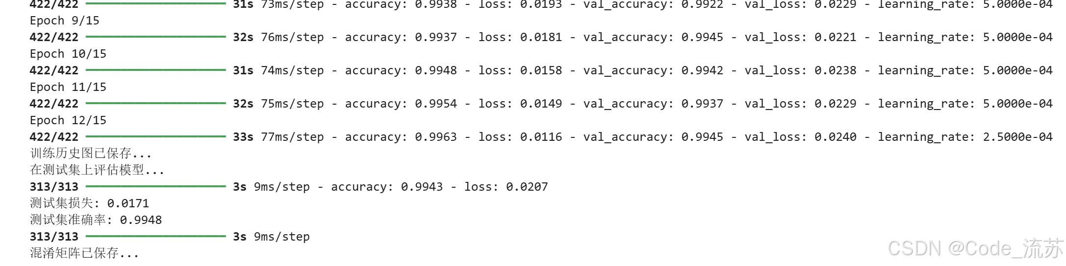
print("训练历史图已保存...")# 7. 评估模型
print("在测试集上评估模型...")
test_loss, test_acc = model.evaluate(x_test, y_test_onehot)
print(f"测试集损失: {test_loss:.4f}")
print(f"测试集准确率: {test_acc:.4f}")# 8. 模型预测
predictions = model.predict(x_test)
predicted_classes = np.argmax(predictions, axis=1)# 9. 混淆矩阵
cm = confusion_matrix(y_test, predicted_classes)
plt.figure(figsize=(10, 8))
sns.heatmap(cm, annot=True, fmt='d', cmap='Blues', xticklabels=range(10), yticklabels=range(10))
plt.xlabel('预测标签')
plt.ylabel('真实标签')
plt.title('混淆矩阵')
plt.savefig('confusion_matrix.png')
plt.close()
print("混淆矩阵已保存...")# 10. 分类报告
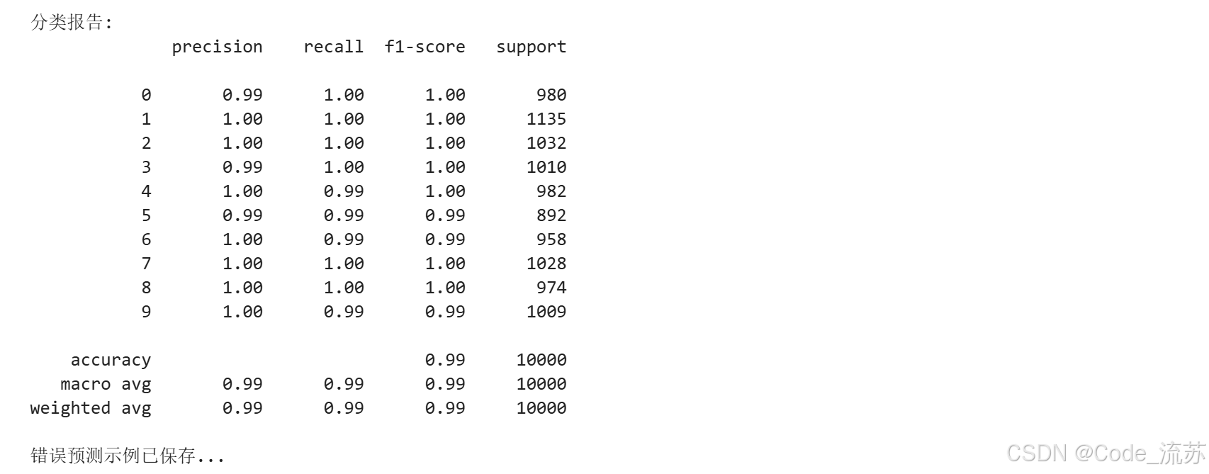
report = classification_report(y_test, predicted_classes)
print("\n分类报告:")
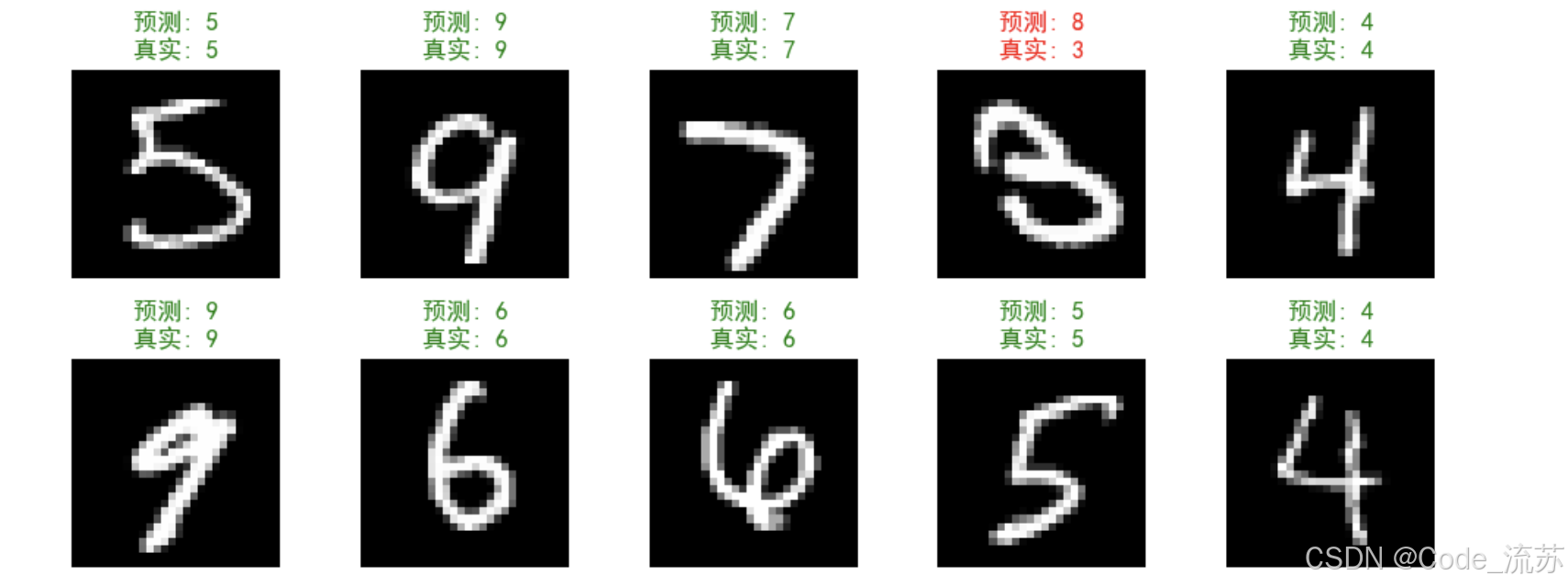
print(report)# 11. 展示错误预测示例
errors = (predicted_classes != y_test)
x_test_errors = x_test[errors]
y_pred_errors = predicted_classes[errors]
y_true_errors = y_test[errors]# 随机选择一些错误预测的样本
n_errors_to_show = min(10, len(x_test_errors))
error_indices = np.random.choice(len(x_test_errors), n_errors_to_show, replace=False)plt.figure(figsize=(12, 6))
for i, idx in enumerate(error_indices):plt.subplot(2, 5, i+1)plt.imshow(x_test_errors[idx].reshape(28, 28), cmap='gray')plt.title(f"预测: {y_pred_errors[idx]}\n真实: {y_true_errors[idx]}", color='red')plt.axis('off')
plt.tight_layout()
plt.savefig('prediction_errors.png')
plt.close()
print("错误预测示例已保存...")# 12. 可视化卷积层输出
def visualize_conv_outputs(model, image):# 创建一个截断模型，只包含前两个卷积层layer_outputs = [layer.output for layer in model.layers if 'conv2d' in layer.name]activation_model = tf.keras.Model(inputs=model.input, outputs=layer_outputs)# 获取激活值activations = activation_model.predict(image.reshape(1, 28, 28, 1))# 绘制激活值plt.figure(figsize=(15, 8))# 原图plt.subplot(1, 3, 1)plt.imshow(image.reshape(28, 28), cmap='gray')plt.title('原始图像')plt.axis('off')# 第一个卷积层的前16个滤波器输出plt.subplot(1, 3, 2)plt.imshow(visualize_filters(activations[0][0, :, :, :16]))plt.title('第一个卷积层输出')plt.axis('off')# 第二个卷积层的前16个滤波器输出plt.subplot(1, 3, 3)plt.imshow(visualize_filters(activations[1][0, :, :, :16]))plt.title('第二个卷积层输出')plt.axis('off')plt.tight_layout()plt.savefig('conv_layer_outputs.png')plt.close()def visualize_filters(activation):# 创建一个网格来可视化滤波器输出n_filters = activation.shape[-1]size = activation.shape[0]# 确定网格尺寸n_cols = 4n_rows = n_filters // n_cols# 创建输出图像display_grid = np.zeros((n_rows * size, n_cols * size))# 填充输出图像for row in range(n_rows):for col in range(n_cols):filter_idx = row * n_cols + colif filter_idx < n_filters:# 将激活值归一化到0-1channel_image = activation[:, :, filter_idx]if channel_image.std() > 0:channel_image = (channel_image - channel_image.mean()) / channel_image.std()channel_image = np.clip(channel_image, -2, 2)channel_image = (channel_image + 2) / 4# 添加到显示网格display_grid[row*size:(row+1)*size, col*size:(col+1)*size] = channel_imagereturn display_grid# 选择一个测试样本进行可视化
sample_idx = np.random.choice(len(x_test))
sample_image = x_test[sample_idx]
visualize_conv_outputs(model, sample_image)
print("卷积层输出可视化已保存...")# 13. 保存模型
model.save('mnist_cnn_model.h5')
print("模型已保存为 'mnist_cnn_model.h5'")print("\n手写数字识别系统训练与评估完成！")

在这里插入图片描述

2. 代码解析

数据预处理：
- 将图像像素值缩放到0-1范围
- 调整形状为(batch_size, 28, 28, 1)，适应CNN输入
- 将标签转换为one-hot编码
CNN架构：
- 两个卷积块，每个包含两个卷积层、批量归一化、池化和Dropout
- 使用了批量归一化（Batch Normalization）来加速训练和提高性能
- 使用了Dropout来防止过拟合
训练技巧：
- 使用早停（Early Stopping）避免过拟合
- 使用学习率降低（ReduceLROnPlateau）在训练停滞时降低学习率
可视化与分析：
- 混淆矩阵：显示模型在不同类别上的表现
- 分类报告：提供精确率、召回率、F1分数等指标
- 卷积层输出可视化：了解CNN如何"看待"图像