混淆矩阵（Confusion Matrix）

        混淆矩阵（Confusion Matrix）是一个用于评估分类模型性能的工具，特别是在机器学习和统计学领域。它展示了模型预测结果与实际结果之间的关系。混淆矩阵通常用于二分类或多分类问题中，但也可以扩展到更多类别的情况。

一、混淆矩阵的基本组成

        对于一个二分类问题，混淆矩阵包含四个元素：

1. 真正例（True Positive, TP）：模型预测为正类，实际也为正类的数量。
2. 假正例（False Positive, FP）：模型预测为正类，实际为负类的数量。
3. 真负例（True Negative, TN）：模型预测为负类，实际也为负类的数量。
4. 假负例（False Negative, FN）：模型预测为负类，实际为正类的数量。

        对于多分类问题，混淆矩阵会扩展为一个方阵，其中每一行代表实际类别，每一列代表预测类别。矩阵中的每个单元格表示实际类别为该行类别，预测类别为该列类别的样本数量。

二、混淆矩阵的用途

        1.评估模型性能

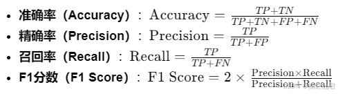
        通过混淆矩阵可以计算出多种性能指标，如准确率（Accuracy）、精确率（Precision）、召回率（Recall）和F1分数（F1 Score）等。

        

import numpy as np
from sklearn.metrics import confusion_matrix# 假设真实标签和预测标签如下：
y_true = np.array([1, 0, 1, 1, 0, 1, 0])
y_pred = np.array([1, 0, 1, 0, 0, 1, 1])# 计算混淆矩阵
cm = confusion_matrix(y_true, y_pred)# 计算TP, TN, FP, FN
TP = cm[1, 1]
TN = cm[0, 0]
FP = cm[0, 1]
FN = cm[1, 0]# 计算性能指标
accuracy = (TP + TN) / (TP + TN + FP + FN)
precision = TP / (TP + FP)
recall = TP / (TP + FN)
f1_score = 2 * (precision * recall) / (precision + recall)print(f"Accuracy: {accuracy:.2f}, Precision: {precision:.2f}, Recall: {recall:.2f}, F1 Score: {f1_score:.2f}")

        这段代码首先计算了混淆矩阵，然后从中提取了TP、TN、FP和FN的值，最后计算了准确率、精确率、召回率和F1分数。       

2.识别模型错误

        混淆矩阵可以帮助识别模型在哪些类别上表现不佳，从而针对性地进行改进。

import matplotlib.pyplot as plt
import seaborn as sns
from sklearn.metrics import confusion_matrix# 假设真实标签和预测标签如下：
y_true = [0, 1, 0, 1, 0, 1, 0, 1]
y_pred = [0, 1, 0, 1, 0, 0, 1, 1]# 创建混淆矩阵
cm = confusion_matrix(y_true, y_pred)# 可视化混淆矩阵
sns.heatmap(cm, annot=True, fmt='d', cmap='Blues')
plt.title('Confusion Matrix')
plt.xlabel('Predicted')
plt.ylabel('True')
plt.show()

        通过可视化混淆矩阵，我们可以直观地看到模型在哪些类别上犯了错误，从而针对性地进行改进。

         3. 平衡类别

        在类别不平衡的情况下，混淆矩阵可以帮助我们理解模型是否倾向于预测多数类。

from sklearn.datasets import make_classification
from sklearn.linear_model import LogisticRegression
from sklearn.model_selection import train_test_split
from sklearn.metrics import classification_report, confusion_matrix# 生成模拟的二分类数据
X, y = make_classification(n_samples=1000, n_features=20, n_informative=2, n_redundant=10, weights=[0.99], random_state=42)
X_train, X_test, y_train, y_test = train_test_split(X, y, test_size=0.2, random_state=42)# 训练一个逻辑回归模型
model = LogisticRegression()
model.fit(X_train, y_train)# 在测试集上预测
y_pred = model.predict(X_test)# 计算混淆矩阵
cm = confusion_matrix(y_test, y_pred)# 打印分类报告，得到精确度、召回率和F1分数等指标
report = classification_report(y_test, y_pred)
print(report)
print(cm)

        这段代码生成了一个类别极度不平衡的数据集，并训练了一个逻辑回归模型。通过打印分类报告和混淆矩阵，我们可以分析模型是否倾向于预测多数类。

三、混淆矩阵的实际应用

        对于二分类问题的混淆矩阵，，我们有一个二分类问题，其中y_true是真实标签，y_pred是模型预测的标签。混淆矩阵显示：

• 真正例（TP）: 2（模型正确预测为正类）
• 假正例（FP）: 1（模型错误预测为正类）
• 真负例（TN）: 3（模型正确预测为负类）
• 假负例（FN）: 1（模型错误预测为负类）

        则有代码如下：

import numpy as np
from sklearn.metrics import confusion_matrix# 真实标签和预测标签
y_true = np.array([1, 0, 1, 1, 0, 1, 0])
y_pred = np.array([1, 0, 1, 0, 0, 1, 1])# 计算混淆矩阵
cm = confusion_matrix(y_true, y_pred)
print("Confusion Matrix:\n", cm)

输出为Confusion Matrix:
 [[2 1]
 [1 3]]

同时对这个进行思维扩散，展示了一个多分类问题，我们使用支持向量机（SVM）对数字识别数据集进行分类，只区分数字9和其他数字。plot_confusion_matrix函数用于绘制混淆矩阵，其中归一化选项可以显示每个类别的预测比例而不是绝对数量。

import matplotlib.pyplot as plt
from sklearn import metrics
from sklearn.model_selection import train_test_split
from sklearn.svm import SVC# 假设digits是加载的数据集
from sklearn.datasets import load_digits
digits = load_digits()
X = digits.data
y = digits.target.copy()
y[digits.target==9] = 1
y[digits.target!=9] = 0X_train, X_test, y_train, y_test = train_test_split(X, y, random_state=666)
svc = SVC(kernel='rbf')
svc.fit(X_train, y_train)
y_pred = svc.predict(X_test)# 绘制混淆矩阵
def plot_confusion_matrix(y_true, y_pred, classes, title='Confusion Matrix', normalize=False):cm = metrics.confusion_matrix(y_true, y_pred)if normalize:cm = cm.astype('float') / cm.sum(axis=1)[:, np.newaxis]plt.imshow(cm, interpolation='nearest', cmap='Blues')plt.title(title)plt.colorbar()tick_marks = np.arange(len(classes))plt.xticks(tick_marks, classes, rotation=45)plt.yticks(tick_marks, classes)fmt = '.2f' if normalize else 'd'thresh = cm.max() / 2.for i, j in np.ndindex(cm.shape):plt.text(j, i, format(cm[i, j], fmt),horizontalalignment="center",color="white" if cm[i, j] > thresh else "black")plt.tight_layout()plt.ylabel('True label')plt.xlabel('Predicted label')plot_confusion_matrix(y_test, y_pred, classes=['not 9', '9'], title='Confusion Matrix for Handwritten Digits')
plt.show()

        其展示了如何在Python中使用sklearn库来计算和可视化混淆矩阵，以及如何从混淆矩阵中提取有用的性能指标。