当前位置：首页 > news >正文

tinyrenderer笔记（上）

news 来源：原创 2025/5/7 6:49:07

tinyrenderer
个人代码仓库：tinyrenderer个人练习代码
参考笔记：从零构建光栅器，tinyrenderer笔记（上） - 知乎

第 1 课：Bresenham 画线算法

Bresenham 画线算法：Bresenham 直线算法 - 知乎

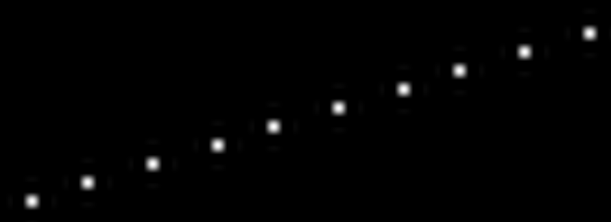
第一次尝试

void line(int x0, int y0, int x1, int y1, TGAImage& image, TGAColor color)
{for (float t = 0.f; t <= 1.f; t += 0.01f){int x = x0 + (x1 - x0) * t;int y = y0 + (y1 - y0) * t;image.set(x, y, color);}
}

利用插值公式，每次使 x、y 的坐标增加一点，简单易懂，模拟的准确度依赖于 t 的大小。

第二次尝试

上面结果过于离散化，将 t 变为 0.01，增加绘制的点数：

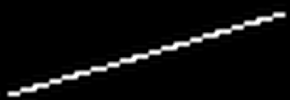
效果变好了，但存在问题：

像素位置（x 与 y）是整数，我们将浮点数截断转化为整数，如果直线比较短，会对同一个 (x,y) 遍历多次，导致了大量重复无意义的绘制。
如果直线过长，t = 0.01 可能还是不够，需要更小的值。

所以我们令 $\Delta x=1$ ，然后根据插值公式计算 y：

void line(int x0, int y0, int x1, int y1, TGAImage& image, TGAColor color)
{for (int x = x0; x <= x1; x++){float t = (x - x0) / (float)(x1 - x0);int y = y0 + (y1 - y0) * t;image.set(x, y, color);}
}

这样不论直线长度为多少，都能绘制出视觉上较为连续的直线。

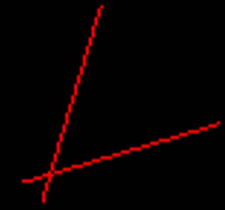
现在一次性绘制 3 条直线：

line(13, 20, 80, 40, image, white); 
line(20, 13, 40, 80, image, red); 
line(80, 40, 13, 20, image, red);

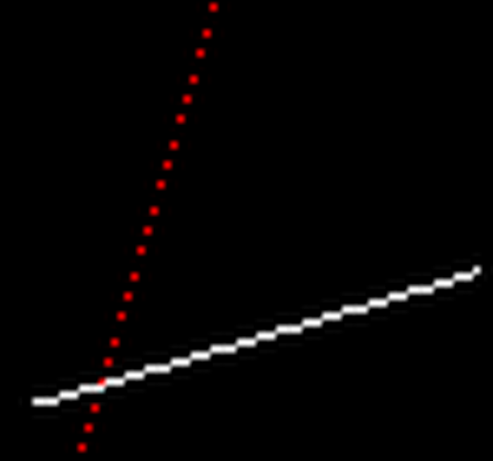
结果并不好：

只存在第一条和第二条直线，第三条红色直线应该覆盖第一条白色直线才对
第二条红色直线过于离散化

先看第一个问题：我们的代码未考虑 x1 > x0 的情况，所以改正一下：

if (x0 > x1)
{std::swap(x0, x1);std::swap(y0, y1);
}

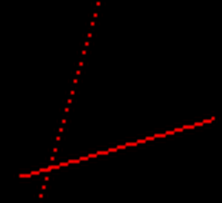
第三次尝试

在看第二个问题：我们现在保证了 $\Delta x=1$ ，但没有保证 $\Delta y \leq 1$ ，当直线斜率 $k > 1$ 时， $\Delta y > 1$ ，从而导致 y 绘制的离散化。

这个问题也很好解决，既然直线斜率 $k > 1$ ，那么我们是不是可以令 $\Delta y=1$ ，然后利用插值公式计算 x 呢？完全没问题：

void line(int x0, int y0, int x1, int y1, TGAImage& image, TGAColor color)
{if (std::abs(x0 - x1) < std::abs(y0 - y1)) {if (y0 > y1){std::swap(x0, x1);std::swap(y0, y1);}for (int y = y0; y <= y1; y++){float t = (y - y0) / (float)(y1 - y0);int x = x0 + (x1 - x0) * t;image.set(x, y, color);}}else{if (x0 > x1){std::swap(x0, x1);std::swap(y0, y1);}for (int x = x0; x <= x1; x++){float t = (x - x0) / (float)(x1 - x0);int y = y0 + (y1 - y0) * t;image.set(x, y, color);}}
}

结果不错，但你会不会发现我们的代码有点太长了，两个 if 分支内的代码高度相似，直觉告诉我们可以将这两个地方合并一下。

动手能力强的小伙伴已经发现了，当 $k > 1$ 时，我们将 x 与 y 交换一下值，在绘制的时候在交换回来就行了：

void line(int x0, int y0, int x1, int y1, TGAImage& image, TGAColor color)
{// 标记 k 是否大于 1bool steep = false;if (std::abs(x0 - x1) < std::abs(y0 - y1)) {// k > 1，交换 x 与 y 的值std::swap(x0, y0);std::swap(x1, y1);steep = true;}if (x0 > x1) {std::swap(x0, x1);std::swap(y0, y1);}for (int x = x0; x <= x1; x++) {float t = (x - x0) / (float)(x1 - x0);int y = y0 + (y1 - y0) * t;steep ? image.set(y, x, color) : image.set(x, y, color);}
}

第四次尝试

以上的代码在不考虑性能的情况下已经表现很好了，接下来的代码都是对性能的优化。

现在我们观察上面的代码，在每次循环中，我们进行了如下的操作：

float t = (x - x0) / (float)(x1 - x0);
int y = y0 + (y1 - y0) * t;
steep ? image.set(y, x, color) : image.set(x, y, color);

我们通过插值得到 y 值，而为了进行插值，我们进行了 3 次浮点运算（一次除法，一次乘法，一次加法）。我们希望减少浮点运算的次数，应该怎么做呢？

其实我们可以不进行插值运算来得到 y 值，我们令 $\Delta x=1$ ，记当前点为 $x_{cur},y_{cur})$ ，前一个点为 $x_{last},y_{last})$ ，可轻易得到以下结论：

$\begin{gathered} y_{cur} = y_{last} + \Delta y\\ \frac{\Delta y}{\Delta x}=k \end{gathered}$

带入 $\Delta x =1$ 可得：

$y_{cur}=y_{last}+k$

在循环迭代之前，我们计算出斜率 $k$ ，然后在每次循环迭代中，我们同时记录 y 值就可以将浮点运算次数降到 1。

void line(int x0, int y0, int x1, int y1, TGAImage& image, TGAColor color)
{// 标记 k 是否大于 1bool steep = false;if (std::abs(x0 - x1) < std::abs(y0 - y1)){// k > 1，交换 x 与 y 的值std::swap(x0, y0);std::swap(x1, y1);steep = true;}if (x0 > x1){std::swap(x0, x1);std::swap(y0, y1);}int dx = x1 - x0;int dy = y1 - y0;// 斜率 kfloat derror = std::abs(dy / float(dx));float y = y0;for (int x = x0; x <= x1; x++) {steep ? image.set(y, x, color) : image.set(x, y, color);y += derror;}
}

在每次循环迭代中，我们只进行了一次浮点加法，显著的提高了效率。但这仍然存在一个问题：image.set 接受的参数类型为整型，将浮点数传入会触发截断操作，例如 1.9 会被认为 1。但我们更希望四舍五入而非直接截断小数位。所以我们用另外一个变量来存储小数部分：

void line(int x0, int y0, int x1, int y1, TGAImage& image, TGAColor color)
{// 标记 k 是否大于 1bool steep = false;if (std::abs(x0 - x1) < std::abs(y0 - y1)){// k > 1，交换 x 与 y 的值std::swap(x0, y0);std::swap(x1, y1);steep = true;}if (x0 > x1){std::swap(x0, x1);std::swap(y0, y1);}int dx = x1 - x0;int dy = y1 - y0;// 斜率 kfloat derror = std::abs(dy / float(dx));// y 的小数部分float error = 0;int y = y0;for (int x = x0; x <= x1; x++) {steep ? image.set(y, x, color) : image.set(x, y, color);error += derror;// 四舍五入if (error > 0.5) {// 判断斜率是否为负y += (y1 > y0 ? 1 : -1);error -= 1.0;}}
}

在上面的代码中，我们用 error 存储小数位，每当 error > 0.5 时我们会将 y 加 1 或减 1。但这又引入了另外一个问题，上面的浮点运算次数又变成了 3 次（一次加法，一次比较，一次减法）。但相比于最开始的 3 次浮点运算（一次除法，一次乘法，一次加法），我们消除了浮点除法与乘法，在浮点运算类型中，乘法与除法也是最耗时的（特别是除法）。

第五次尝试

观察上面的代码，浮点运算的对象都有 error，思考 error 这个浮点数在这里的作用是什么？它的作用只是决定了 y 是否变化 1，所以只要保证 y 变化的时机没有发生改变，那么 error 每次递增 k，还是递增多少，都对结果没有影响。

请看下面 3 个浮点运算式的推导（ $dy=y_1-y_0$ ， $dx=x_1-x_0$ ）：

$\begin{gathered} error = error + \frac{d y}{d x}\\ error > 0.5\\ error = error - 1.0 \end{gathered}$

等式两边同乘 $2 d x$ ：

$\begin{gathered} 2error*dx = 2error*dx + 2dy\\ 2error*dx > dx\\ 2error*dx= 2error*dx - 2dx \end{gathered}$

所以满足 $2 error * d x > d x$ 就相当于满足了 $error > 0.5$ ，y 是否变化的时机也就没有发生变化。这里我们记 $2 error * d x$ 为 error2，3 个浮点运算式也就变成了：

$\begin{gathered} error2 = error2 + 2dy\\ error2 > dx\\ error2 = error2 - 2dx \end{gathered}$

我们这么做的意义是什么？观察这 3 个浮点运算式，你会发现与 error2 计算相关的变量都变成了整数，这就意味着 error2 也是一个整数！所以我们直接将浮点运算次数降到了 0！

void line(int x0, int y0, int x1, int y1, TGAImage& image, TGAColor color)
{// 标记 k 是否大于 1bool steep = false;if (std::abs(x0 - x1) < std::abs(y0 - y1)){// k > 1，交换 x 与 y 的值std::swap(x0, y0);std::swap(x1, y1);steep = true;}if (x0 > x1){std::swap(x0, x1);std::swap(y0, y1);}int dx = x1 - x0;int dy = y1 - y0;int derror2 = std::abs(dy) * 2;int error2 = 0;int y = y0;for (int x = x0; x <= x1; x++) {steep ? image.set(y, x, color) : image.set(x, y, color);error2 += derror2;if (error2 > dx) {y += (y1 > y0 ? 1 : -1);error2 -= dx * 2;}}
}

第六次尝试

这个是在 issues 中被提出来的，主要思想是减少循环迭代时的分支：

steep ? image.set(y, x, color) : image.set(x, y, color);
y += (y1 > y0 ? 1 : -1);

将上面这两个分支代码提到循环迭代之前：

void line(int x0, int y0, int x1, int y1, TGAImage& image, TGAColor color)
{// 标记 k 是否大于 1bool steep = false;if (std::abs(x0 - x1) < std::abs(y0 - y1)){// k > 1，交换 x 与 y 的值std::swap(x0, y0);std::swap(x1, y1);steep = true;}if (x0 > x1){std::swap(x0, x1);std::swap(y0, y1);}int dx = x1 - x0;int dy = y1 - y0;int derror2 = std::abs(dy) * 2;int error2 = 0;int y = y0;const int yincr = (y1 > y0 ? 1 : -1);if (steep){for (int x = x0; x <= x1; x++){image.set(y, x, color);error2 += derror2;if (error2 > dx){y += yincr;error2 -= dx * 2;}}}else{for (int x = x0; x <= x1; x++){image.set(x, y, color);error2 += derror2;if (error2 > dx){y += yincr;error2 -= dx * 2;}}}
}

So it’s a pretty impressive speedup to eliminate the branch instruction inside a loop.

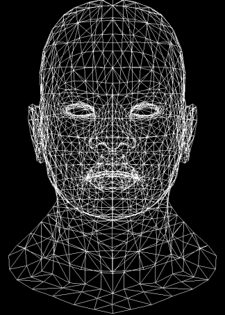
线框渲染

引入了一个 modle 类，用于从 obj 文件中读取点与面的信息。核心代码也很简单：

Model::Model(const char *filename) : verts_(), faces_() {std::ifstream in;in.open (filename, std::ifstream::in);if (in.fail()) return;std::string line;while (!in.eof()) {std::getline(in, line);std::istringstream iss(line.c_str());char trash;if (!line.compare(0, 2, "v ")) {iss >> trash;Vec3f v;for (int i=0;i<3;i++) iss >> v.raw[i];verts_.push_back(v);} else if (!line.compare(0, 2, "f ")) {std::vector<int> f;int itrash, idx;iss >> trash;while (iss >> idx >> trash >> itrash >> trash >> itrash) {idx--; // in wavefront obj all indices start at 1, not zerof.push_back(idx);}faces_.push_back(f);}}std::cerr << "# v# " << verts_.size() << " f# "  << faces_.size() << std::endl;
}

model 存储的点位于模型空间中，坐标范围为 $[- 1, 1]$ 。我们需要将其转换到屏幕空间范围内： $[0, w i d t h]$ 与 $[0, h e i g h t]$ 。现在我们只是在一个平面上绘制直线，所以不考虑深度即 z 坐标的影响。

auto* model = new Model("obj/african_head.obj");
for (int i = 0; i < model->nfaces(); i++) 
{std::vector<int> face = model->face(i);for (int j = 0; j < 3; j++) {// face 存储的是 vertex 的序号Vec3f v0 = model->vert(face[j]);Vec3f v1 = model->vert(face[(j + 1) % 3]);int x0 = (v0.x + 1.) * width / 2.;int y0 = (v0.y + 1.) * height / 2.;int x1 = (v1.x + 1.) * width / 2.;int y1 = (v1.y + 1.) * height / 2.;line(x0, y0, x1, y1, image, white);}
}

本次代码提交记录：

第 2 课：三角形光栅化和背面剔除

老式方法：线扫描

绘制一个二维三角形，但不填充内部区域的代码很简单：

void triangle(Vec2i t0, Vec2i t1, Vec2i t2, TGAImage& image, TGAColor color)
{line(t0.x, t0.y, t1.x, t1.y, image, color);line(t1.x, t1.y, t2.x, t2.y, image, color);line(t2.x, t2.y, t0.x, t0.y, image, color);
}// ......
Vec2i t0[3] = {Vec2i(10, 70),   Vec2i(50, 160),  Vec2i(70, 80)}; 
Vec2i t1[3] = {Vec2i(180, 50),  Vec2i(150, 1),   Vec2i(70, 180)}; 
Vec2i t2[3] = {Vec2i(180, 150), Vec2i(120, 160), Vec2i(130, 180)}; 
triangle(t0[0], t0[1], t0[2], image, red); 
triangle(t1[0], t1[1], t1[2], image, white); 
triangle(t2[0], t2[1], t2[2], image, green);

三角形内部的填充可以用 vertex 也可以用 line，最直观的思路就是用水平或垂直的 line 去填充：

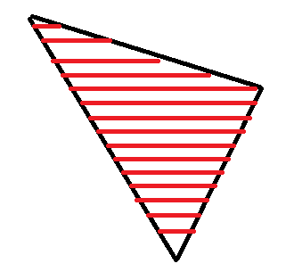
假设我们从下往上绘制，令 $\Delta y=1$ 左侧的端点可直接通过直线的解析方程或者插值公式获得，而右侧的端点跨过了两条直线，我们无法通过一个解析方程表示两条直线，所以我们需要将整个三角形的填充分成两步，一次填充下半部分，一次填充上半部分：

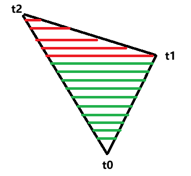
void triangle(Vec2i t0, Vec2i t1, Vec2i t2, TGAImage& image, TGAColor color)
{// 排序顶点, t0.y < t1.y < t2.yif (t0.y > t1.y) std::swap(t0, t1);if (t0.y > t2.y) std::swap(t0, t2);if (t1.y > t2.y) std::swap(t1, t2);int total_height = t2.y - t0.y;// 下半部分for (int y = t0.y; y <= t1.y; y++) {int segment_height = t1.y - t0.y + 1;float alpha = (float)(y - t0.y) / total_height;float beta = (float)(y - t0.y) / segment_height;Vec2i A = t0 + (t2 - t0) * alpha;Vec2i B = t0 + (t1 - t0) * beta;if (A.x > B.x) std::swap(A, B);for (int j = A.x; j <= B.x; j++) {image.set(j, y, color);}}// 上半部分for (int y = t1.y; y <= t2.y; y++) {int segment_height = t2.y - t1.y + 1;float alpha = (float)(y - t0.y) / total_height;float beta = (float)(y - t1.y) / segment_height;Vec2i A = t0 + (t2 - t0) * alpha;Vec2i B = t1 + (t2 - t1) * beta;if (A.x > B.x) std::swap(A, B);for (int j = A.x; j <= B.x; j++) {image.set(j, y, color);}}
}

可将两个循环合并到一起：

void triangle(Vec2i t0, Vec2i t1, Vec2i t2, TGAImage &image, TGAColor color) { if (t0.y==t1.y && t0.y==t2.y) return;// 不管退化的三角形if (t0.y>t1.y) std::swap(t0, t1); if (t0.y>t2.y) std::swap(t0, t2); if (t1.y>t2.y) std::swap(t1, t2); int total_height = t2.y-t0.y; for (int i=0; i<total_height; i++) { bool second_half = i>t1.y-t0.y || t1.y==t0.y; int segment_height = second_half ? t2.y-t1.y : t1.y-t0.y; float alpha = (float)i/total_height; float beta  = (float)(i-(second_half ? t1.y-t0.y : 0))/segment_height;Vec2i A =               t0 + (t2-t0)*alpha; Vec2i B = second_half ? t1 + (t2-t1)*beta : t0 + (t1-t0)*beta; if (A.x>B.x) std::swap(A, B); for (int j=A.x; j<=B.x; j++) { image.set(j, t0.y+i, color); } } 
}

区域填充算法

核心思想是遍历三角形的包围盒，然后对包围盒内的每个 vertex 判断是否在三角形内部，如果在，那么就绘制这个点：

triangle(vec2 points[3]) { vec2 bbox[2] = find_bounding_box(points); for (each pixel in the bounding box) { if (inside(points, pixel)) { put_pixel(pixel); } } 
}

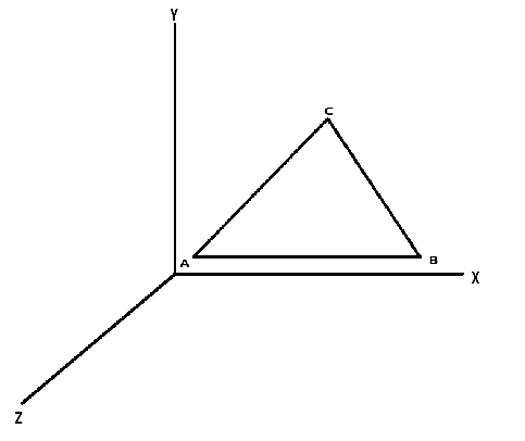
得到三角形的包围盒十分容易，这里唯一的难点在于如何判断一个点是否在三角形内部，设三角形三个顶点为 $A$ 、 $B$ 、 $C$ ，给定任意点 $P$ ，下面列出了常用的四种方法：

面积法

将点 $P$ 与三角形的三个顶点 $A, B, C$ 连接，形成三个小三角形 $P A B$ 、 $PBC$ 、 $PC A$ 。如果 $P$ 在三角形 $A BC$ 内部，则这三个小三角形的面积之和等于原三角形 $A BC$ 的面积。

常用的面积公式（行列式形式）：

$\text{S}(A,B,C)=\frac{1}{2}\vert x_A(y_B - y_C)+x_B(y_C - y_A)+x_C(y_A - y_B)\vert$

需要计算 4 个三角形的面积（原三角形 + 3 个子三角形），计算量较大。

射线法

从点 $P$ 向任意方向（如正右方）发射一条射线，统计与三角形边的 交点数。若交点数为奇数，则 $P$ 在三角形内部；否则在外部。对三角形来说，需要 3 次线段相交判断，计算量较大。但该方法适用于任意多边形，通用性强。

叉积法（同向法）

通过向量叉积判断点 $P$ 是否在三角形的 同一侧。若三角形顶点按 顺时针或逆时针顺序排列，则 $P$ 必须在三角形三条边的 同一侧（例如，始终在左侧或右侧）。

构建向量：

$\overrightarrow{AB}=B-A$
$\overrightarrow{AC}=C-A$
$\overrightarrow{AP}=P-A$

计算叉积：

$c1=\overrightarrow{AB} \times \overrightarrow{AP}$
$c2=\overrightarrow{BC} \times \overrightarrow{BP}$
$c3=\overrightarrow{CA} \times \overrightarrow{CP}$

然后检查 $c 1$ 、 $c 2$ 、 $c 3$ 符号是否一致。此方法仅需 3 次叉积计算，运算量小（乘法和减法）。且无需浮点平方根运算，精度较高。

1. 二维向量叉乘

对于二维向量 $a = (a_1, a_2)$ 和 $b = (b_1, b_2)$ ，叉乘结果为标量：

$\times b = a_1 b_2 - a_2 b_1$

几何意义：
• 绝对值表示两向量张成的平行四边形面积。
• 符号表示方向：正值为 $b$ 在 $a$ 的逆时针方向，负值则为顺时针

2. 三维向量叉乘

对于三维向量 $a = (a_1, a_2, a_3)$ 和 $b = (b_1, b_2, b_3)$ ，叉乘结果为向量：

$\times b = \left ( a_2 b_3 - a_3 b_2, \ a_3 b_1 - a_1 b_3, \ a_1 b_2 - a_2 b_1 \right)$

或用行列式表示：
$\times b = \begin{vmatrix} \mathbf{i} & \mathbf{j} & \mathbf{k} \\ a_1 & a_2 & a_3 \\ b_1 & b_2 & b_3 \end{vmatrix}$

几何意义：
• 模长为两向量张成的平行四边形面积。
• 方向由右手定则确定，垂直于原向量所在平面。

重心坐标法

首先了解重心坐标的知识：计算机图形学补充1：重心坐标(barycentric coordinates)详解及其作用 - 知乎

点 $P$ 的重心坐标（Barycentric Coordinates）是相对于三角形 $△ A BC$ 的参数，表示为 $(u, v, w)$ ，满足：

$P = w A + v B + u C 且 u + v + w = 1$

也可以理解为以 $A$ 为原点，将 $\overrightarrow{AC}$ 与 $\overrightarrow{AB}$ 当作基向量来线性表示 $\overrightarrow{AP}$ ：

$\begin{aligned} P&=wA+vB+uC\\ P&=(1-u-v)A+vB+uC\\ P&=u(C-A)+v(B-A)+A\\ P-A&=u(C-A)+v(B-A)\\ \overrightarrow{AP}&=u\overrightarrow{AC}+v\overrightarrow{AB} \end{aligned}$

$p$ 点在三角形内部的充分必要条件是： $1 >= u >= 0, 1 >= v >= 0, u + v <= 1$ 。

求解方法一

求解 $u, v, w$ 的方法有很多，你可以直接带入坐标用以下的公式得到（推导请参考上面的链接）：

$\begin{align*} u &= \frac{(y_a - y_b)x+(x_b - x_a)y + x_ay_b - x_by_a}{(y_a - y_b)x_c+(x_b - x_a)y_c + x_ay_b - x_by_a},\\ v &= \frac{(y_a - y_c)x+(x_c - x_a)y + x_ay_c - x_cy_a}{(y_a - y_c)x_b+(x_c - x_a)y_b + x_ay_c - x_cy_a},\\ w &= 1 - u - v. \end{align*}$

求解方法二

也可以将 $\overrightarrow{AP}=u\overrightarrow{AC}+v\overrightarrow{AB}$ 等式两边同时点乘 $\overrightarrow{AC}$ 与 $\overrightarrow{AB}$ ：

$\begin{align*} \overrightarrow{AP}\cdot\overrightarrow{AC}&=(u\overrightarrow{AC}+v\overrightarrow{AB})\cdot\overrightarrow{AC}\\ \overrightarrow{AP}\cdot\overrightarrow{AB}&=(u\overrightarrow{AC}+v\overrightarrow{AB})\cdot\overrightarrow{AB} \end{align*}$

解方程得到：

$\begin{align*} u&=\frac{(\overrightarrow{AB}\cdot\overrightarrow{AB})*(\overrightarrow{AP}\cdot\overrightarrow{AC})-(\overrightarrow{AC}\cdot\overrightarrow{AB})*(\overrightarrow{AP}\cdot\overrightarrow{AB})}{(\overrightarrow{AC}\cdot\overrightarrow{AC})*(\overrightarrow{AB}\cdot\overrightarrow{AB})-(\overrightarrow{AC}\cdot\overrightarrow{AB})*(\overrightarrow{AB}\cdot\overrightarrow{AC})}\\ v&=\frac{(\overrightarrow{AC}\cdot\overrightarrow{AC})*(\overrightarrow{AP}\cdot\overrightarrow{AB})-(\overrightarrow{AC}\cdot\overrightarrow{AB})*(\overrightarrow{AP}\cdot\overrightarrow{AC})}{(\overrightarrow{AC}\cdot\overrightarrow{AC})*(\overrightarrow{AB}\cdot\overrightarrow{AB})-(\overrightarrow{AC}\cdot\overrightarrow{AB})*(\overrightarrow{AB}\cdot\overrightarrow{AC})} \end{align*}$

此公式也可计算三维空间下的重心坐标

求解方法三

也可像原教程一样推导表达式的几何意义：

$\begin{cases} u\overrightarrow{AC}_x + v\overrightarrow{AB}_x + \overrightarrow{PA}_x = 0 \\ u\overrightarrow{AC}_y + v\overrightarrow{AB}_y + \overrightarrow{PA}_y = 0 \end{cases}$

写成矩阵形式：

$\begin{cases} \begin{bmatrix} u & v & 1 \end{bmatrix} \begin{bmatrix} \overrightarrow{AC}_x \\ \overrightarrow{AB}_x \\ \overrightarrow{PA}_x \end{bmatrix} = 0 \\ \begin{bmatrix} u & v & 1 \end{bmatrix} \begin{bmatrix} \overrightarrow{AC}_y \\ \overrightarrow{AB}_y \\ \overrightarrow{PA}_y \end{bmatrix} = 0 \end{cases}$

可以认为向量 $(u, v, 1)$ 与 $(\overrightarrow{AC}_x , \overrightarrow{AB}_x , \overrightarrow{PA}_x)$ 、 $b=(\overrightarrow{AC}_y , \overrightarrow{AB}_y , \overrightarrow{PA}_y)$ 垂直。若 $A, B, C$ 三点不共线，则 $a$ 与 $b$ 不可能共线，则可推导出：

$(\overrightarrow{AC}_x , \overrightarrow{AB}_x , \overrightarrow{PA}_x) \times (\overrightarrow{AC}_y , \overrightarrow{AB}_y , \overrightarrow{PA}_y) = k(u,v,1)$

若你将两个向量叉积结果进行展开，然后带入表达式，你可以得到：

$a \times b = (u D, v D, D) = D (u, v, 1)$

其中 $\overrightarrow{AC}_x \overrightarrow{AB}_y - \overrightarrow{AB}_x \overrightarrow{AC}_y$ ， $D$ 是向量 $\overrightarrow{AB}$ 与 $\overrightarrow{AC}$ 的二维叉积（即行列式），表示两向量构成的平行四边形的有向面积。由于 ABC 是三角形， $\overrightarrow{AB}$ 与 $\overrightarrow{AC}$ 不共线，因此 $\neq 0$ 。所以当 $\times b$ 的第三个分量为 $0$ 时，代表三角形 ABC 退化成了一条直线。

算法实现

上面的四种方法综合对比下来，叉积法的运算速度最快，重心坐标法其次。在图形渲染中，最常用的方法也是这两种。这里我们选用重心坐标法，因为重心坐标不仅可用来判断点 $P$ 是否在三角形内部，还可以用它来插值求得一些顶点属性。

下面是求点 P 重心坐标的代码：

Vec3f barycentric(Vec2f A, Vec2f B, Vec2f C, Vec2f P)
{Vec3f a = { C.x - A.x, B.x - A.x, A.x - P.x };Vec3f b = { C.y - A.y, B.y - A.y, A.y - P.y };Vec3f u = a ^ b;// 三角形退化if (IsNearlyZero(u.z)){return Vec3f(-1, 1, 1);}return Vec3f(1.f - (u.x + u.y) / u.z, u.y / u.z, u.x / u.z);
}

区域填充算法：

void triangle(Vec2i t0, Vec2i t1, Vec2i t2, TGAImage& image, TGAColor color)
{// 包围盒范围Vec2i bboxmin(image.get_width() - 1, image.get_height() - 1);Vec2i bboxmax(0, 0);bboxmin.x = std::min({ bboxmin.x, t0.x, t1.x, t2.x });bboxmin.y = std::min({ bboxmin.y, t0.y, t1.y, t2.y });bboxmax.x = std::max({ bboxmax.x, t0.x, t1.x, t2.x });bboxmax.y = std::max({ bboxmax.y, t0.y, t1.y, t2.y });Vec2i P;for (int x = bboxmin.x; x <= bboxmax.x; x++){for (int y = bboxmin.y; y <= bboxmax.y; y++){P = Vec2i(x, y);Vec3f bc_screen = barycentric(t0, t1, t2, P);if (bc_screen.x < 0 || bc_screen.y < 0 || bc_screen.z < 0) continue;image.set(x, y, color);}}
}

Flat shading

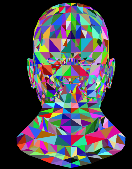
第一课中，我们用线条绘制了模型的框架，现在让我们用随机颜色填充这个模型：

for (int i = 0; i < model->nfaces(); i++)
{std::vector<int> face = model->face(i);Vec2i screen_coords[3];for (int j = 0; j < 3; j++){Vec3f model_coords = model->vert(face[j]);// 模型空间坐标转化为屏幕空间坐标（此处模型空间就相当于世界空间）screen_coords[j] = Vec2i((model_coords.x + 1.0) * width / 2.0, (model_coords.y + 1.0) * height / 2.0);}triangle(screen_coords[0], screen_coords[1], screen_coords[2], image, TGAColor(rand() % 255, rand() % 255, rand() % 255, 255));
}

现在我们将随机颜色换成光照，采用 Flat shading，三角面内的所有点使用相同的法线，法线用三角形顶点向量叉乘获得：

$\vec{n}=\overrightarrow{AB} \times \overrightarrow{AC}$

OBJ 文件中的面默认顶点顺序通常为逆时针排列，用于表示正面（法线朝屏幕外，符合右手定则），所以面法向量应该用 $\overrightarrow{AB} \times \overrightarrow{AC}$ 。

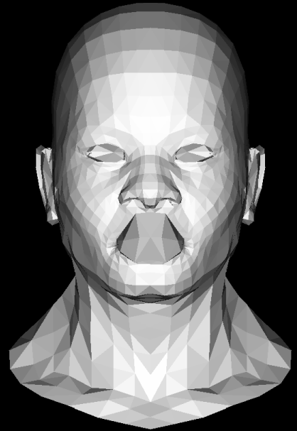
此处只考虑漫反射光照： $intensity=n\cdot light\_dir$ ，但需要注意此处的 $light\_dir$ 需要反向，是着色点朝向光源位置，而非~~光源位置朝向着色点~~。所以实际公式为： $intensity=n\cdot -light\_dir$ 。

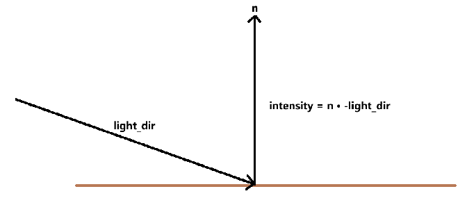
我们使用定向光源 Vec3f light_dir(0, 0, -1)，代码如下：

Vec3f light_dir(0, 0, -1); // define light_dir
for (int i = 0; i < model->nfaces(); i++)
{std::vector<int> face = model->face(i);Vec2i screen_coords[3];Vec3f model_coords;for (int j = 0; j < 3; j++){Vec3f model_coords = model->vert(face[j]);// 模型空间坐标转化为屏幕空间坐标（此处模型空间就相当于世界空间）screen_coords[j] = Vec2i((model_coords.x + 1.0) * width / 2.0, (model_coords.y + 1.0) * height / 2.0);}Vec3f n = (model->vert(face[1]) - model->vert(face[0])) ^ (model->vert(face[2]) - model->vert(face[0]));n.normalize();float intensity = -(n * light_dir);if (intensity > 0) {triangle(screen_coords[0], screen_coords[1], screen_coords[2], image, TGAColor(intensity * 255, intensity * 255, intensity * 255, 255));}
}

点积也可以为负数，代表该三角面背向光源，我们可以将其剔除而不绘制，这称为背向面剔除（Back-face culling）。

本次代码提交记录：

第 3 课：Z-Buffer

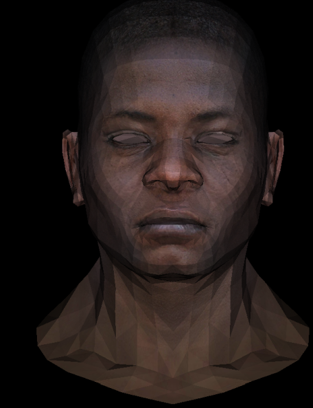
第 2 次课最后绘制出的模型，嘴唇被嘴巴内腔所覆盖。嘴巴内腔应该隐藏在嘴唇之后，不应该被我们直接观察到，除非模型张开了嘴巴。不能被直接观察到的表面被称为隐藏面，我们需要一种算法来进行隐藏面消除。

教程采用的是 Z-Buffer 算法来进行隐藏面消除，思路很简单：为每个像素记录最近（离观察者）的深度值，确保渲染时只显示距离观察者最近的物体表面。

triangle(vec3 points[3]) { vec2 bbox[2] = find_bounding_box(points); for (each pixel in the bounding box) { if (inside(points, pixel)) {// 使用重心坐标对三角形三个顶点的z值进行插值，得到points的z值points.depth = lerp(points[3])if(points.depth < zbuffer.depth){zbuffer.depth = points.depthput_pixel(pixel);} } } 
}

唯一需要注意的是如何得到三角形内部点的深度值，而这就是我们前面采用重心坐标法判断点是否在三角形内部的原因，此时我们已经有了点 P 的重心坐标 $(w, v, u)$ ，观察重心坐标的表达式：

$(x, y) = w A + v B + u C$

若你将顶点位置替换为其它属性，那么你就会发现，重心坐标可以合理的得到三个顶点某个属性的平均。所以点 P 的深度值为：

P.z = bc_screen.x * t0.z + bc_screen.y * t1.z + bc_screen.z * t2.z;

同时还需要注意一个地方由于 z 轴是朝向屏幕外的，所以物体离屏幕越远（深度越深），z 值越小；离屏幕越近（深度越浅），z 值越大。

void triangle(Vec3f t0, Vec3f t1, Vec3f t2, float* zbuffer, TGAImage& image, TGAColor color)
{// 包围盒范围Vec2f bboxmin(image.get_width() - 1, image.get_height() - 1);Vec2f bboxmax(0, 0);bboxmin.x = std::min({ bboxmin.x, t0.x, t1.x, t2.x });bboxmin.y = std::min({ bboxmin.y, t0.y, t1.y, t2.y });bboxmax.x = std::max({ bboxmax.x, t0.x, t1.x, t2.x });bboxmax.y = std::max({ bboxmax.y, t0.y, t1.y, t2.y });Vec3f P;for (int x = bboxmin.x; x <= bboxmax.x; x++){for (int y = bboxmin.y; y <= bboxmax.y; y++){P = Vec3f(x, y, 0);Vec3f bc_screen = barycentric(t0, t1, t2, P);if (bc_screen.x < 0 || bc_screen.y < 0 || bc_screen.z < 0) continue;// 重心坐标插值P.z = bc_screen.x * t0.z + bc_screen.y * t1.z + bc_screen.z * t2.z;if (P.z > zbuffer[int(x + y * width)]){zbuffer[int(x + y * width)] = P.z;image.set(x, y, color);}}}
}

纹理

现在的渲染结果假定三角面的基础颜色是白色，是时候引入纹理贴图了。obj 文件存储了每个顶点的纹理坐标（以 vt 开头），修改我们的 model 类，以存储纹理坐标：

class Model {
private:std::vector<Vec3f> verts_; // 所有顶点std::vector<Vec2f> vertsTexture_; // 所有纹理std::vector<std::vector<int> > facesV_; // 面-顶点std::vector<std::vector<int> > facesVT_; // 面-纹理
public:Model(const char *filename);~Model();int nverts();int nfaces();Vec3f vert(int i);// 获得顶点坐标Vec2f textureCoor(int i);// 获得纹理坐标std::vector<int> face_v(int idx);std::vector<int> face_vt(int idx);
};

增加了存储纹理坐标所需的数组，cpp 文件重要看构造函数，增加了读取纹理坐标的判断语句：

 while (!in.eof()) {std::getline(in, line);std::istringstream iss(line.c_str());char trash;if (!line.compare(0, 2, "v ")) {iss >> trash;Vec3f v;for (int i=0;i<3;i++) iss >> v.raw[i];verts_.push_back(v);} else if (!line.compare(0, 2, "f ")) {std::vector<int> f_v;std::vector<int> f_vt;int itrash, vIdx, vtIdx;iss >> trash;while (iss >> vIdx >> trash >> vtIdx >> trash >> itrash) {vIdx--; // in wavefront obj all indices start at 1, not zerovtIdx--;f_v.push_back(vIdx);f_vt.push_back(vtIdx);}facesV_.push_back(f_v);facesVT_.push_back(f_vt);}else if (!line.compare(0, 4, "vt  ")){iss >> trash;iss >> trash;Vec3f v;for (int i = 0;i < 3;i++) iss >> v.raw[i];vertsTexture_.emplace_back(v[0], v[1]);}}

TGAImage 新增了一个函数，用于采样贴图：

// 输入纹理坐标[0,1]
TGAColor TGAImage::texture(float x, float y)
{if (!data || x < 0 || y < 0) {return TGAColor();}double int_part;// 获得小数部分，确保 <= 1x = std::modf(x, &int_part);y = std::modf(y, &int_part);return get(x * width, y * height);
}

main.cpp 增加了一个顶点信息类：

struct VertexInfo
{Vec3f location;Vec2f textureCoor;
};

在 triangle 函数里面，会根据三个顶点插值得到内部点的纹理坐标，然后去贴图中采样得到颜色值：

void triangle(VertexInfo t0, VertexInfo t1, VertexInfo t2, float* zbuffer, TGAImage& res, TGAImage& tex, float light)
{// 包围盒范围Vec2f bboxmin(res.get_width() - 1, res.get_height() - 1);Vec2f bboxmax(0, 0);bboxmin.x = std::min({ bboxmin.x, t0.location.x, t1.location.x, t2.location.x });bboxmin.y = std::min({ bboxmin.y, t0.location.y, t1.location.y, t2.location.y });bboxmax.x = std::max({ bboxmax.x, t0.location.x, t1.location.x, t2.location.x });bboxmax.y = std::max({ bboxmax.y, t0.location.y, t1.location.y, t2.location.y });Vec3f P;for (int x = bboxmin.x; x <= bboxmax.x; x++){for (int y = bboxmin.y; y <= bboxmax.y; y++){P = Vec3f(x, y, 0);Vec3f bc_screen = barycentric(t0.location, t1.location, t2.location, P);if (bc_screen.x < 0 || bc_screen.y < 0 || bc_screen.z < 0) continue;// 重心坐标插值P.z = bc_screen.x * t0.location.z + bc_screen.y * t1.location.z + bc_screen.z * t2.location.z;if (P.z > zbuffer[int(x + y * width)]){zbuffer[int(x + y * width)] = P.z;Vec2f texCoor = t0.textureCoor * bc_screen.x + t1.textureCoor * bc_screen.y + t2.textureCoor * bc_screen.z;TGAColor diffuse = tex.texture(texCoor.x, texCoor.y);res.set(x, y, TGAColor(diffuse.r * light, diffuse.g * light, diffuse.b * light, 255));}}}
}

main 函数：

for (int i = 0; i < model->nfaces(); i++)
{std::vector<int> face_v = model->face_v(i);std::vector<int> face_vt = model->face_vt(i);VertexInfo vertex[3];for (int j = 0; j < 3; j++){vertex[j].textureCoor = model->textureCoor(face_vt[j]);Vec3f model_coords = model->vert(face_v[j]);// 模型空间坐标转化为屏幕空间坐标（此处模型空间就相当于世界空间）vertex[j].location = Vec3f((model_coords.x + 1.0) * width / 2.0, (model_coords.y + 1.0) * height / 2.0, model_coords.z);}Vec3f n = (model->vert(face_v[1]) - model->vert(face_v[0])) ^ (model->vert(face_v[2]) - model->vert(face_v[0]));n.normalize();float intensity = -(n * light_dir);if (intensity > 0) {triangle(vertex[0], vertex[1], vertex[2], zbuffer, result, texture, intensity);}
}