Matplotlib核心课程-2

4.1 数据加载、储存

4.1.1 从数据文件读取数据

导入支持库：

import numpy as np

from pandas import Series,DataFrame

import pandas as pd

从csv文件读取数据，一般方法：

pd.read_csv('../data/ex1.csv',encoding='gbk')

从csv文件读取数据，去掉头部：

pd.read_csv('../data/ex1.csv',encoding='gbk',header=None)

读取数据，设置头部名称：

colnames = ['商品编号','进货价格(元)','销售价格(元)','销售数量','商品名称']

pd.read_csv('../data/ex1.csv',encoding='gbk',names=colnames)

4.1.2 为读取数据添加索引

添加一级索引：

pd.read_csv('../data/ex1.csv',encoding='gbk',names=colnames,index_col='商品编号')

添加多级索引：

pd.read_csv('../data/csv_mindex.csv',encoding='GBK',index_col=['生产厂商','产品类别'])

4.1.3 读取文件并筛选行

直接读取数据：

pd.read_csv('../data/ex4.csv',encoding='gbk')

设置跳过数据行：

pd.read_csv('../data/ex4.csv',encoding='gbk',skiprows=[0,2,3])

4.1.4设置读取行数

pd.read_csv('../data/ex5.csv')

选择前30行数据：

pd.read_csv('../data/ex5.csv',nrows=30)

4.1.5写csv文件

首先现读取一个文件:

data = pd.read_csv('../data//ex6.csv',encoding='gbk')

data

简单写入文件：

data.to_csv('out1.csv',encoding='UTF8')

4.1.6 写入文件，设置写入参数

data.to_csv('out3.csv',encoding='UTF8',na_rep='NULL',index=False,header=False)

4.1.7 读取数据库

此处只列出连接方法，不做连通测试

导入支持库：

import pymysql

如果提示没有这个模块，请先安装：!pip install pymysql

链接数据库读取数据表：

conn = pymysql.connect(host='localhost',user='root',password='123456',db='employees',charset='utf8')

sql = 'select * from departments'

df = pd.read_sql(sql,conn)

df

4.2 数据规整

4.2.1 导入支持库

import numpy as np

from pandas import Series,DataFrame

import pandas as pd

4.2.2 创建原始数据

data = DataFrame({'k1': ['one'] * 3 + ['two'] * 4,'k2': [1, 1, 2, 3, 3, 4, 4]})

data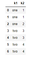

4.2.3 检查重复

data.duplicated()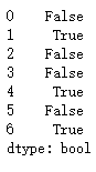

4.2.4 去除重复

data.drop_duplicates()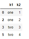

4.2.5 添加一列新的数据

data['v1'] = range(7)

data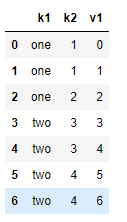

4.2.6 按照k1列为标准，去重

data.drop_duplicates(['k1'])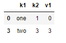

4.2.7 利用映射进行数据转换-创建实验数据

data = DataFrame({'food': ['bacon', 'pulled pork', 'bacon', 'Pastrami', 'corned beef', 'Bacon', 'pastrami', 'honey ham', 'nova lox'], 'ounces': [4, 3, 12, 6, 7.5, 8, 3, 5, 6]}) 

data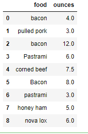

4.2.8 创建映射关系替换数据

meat_to_animal = {'bacon': 'pig','pulled pork': 'pig','pastrami': 'cow','corned beef': 'cow','honey ham': 'pig','nova lox': 'salmon'}

data['animal'] = data['food'].map(meat_to_animal)

data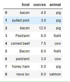

4.2.9 利用函数进行数据转换-调用str.lower函数替换为小写

data['animal'] = data['food'].map(str.lower).map(meat_to_animal) 

data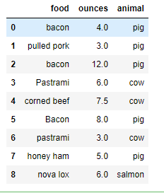

4.2.10 替换值-创建实验数据

data = Series([77., -1., 31., -1., -2., 5.]) 

data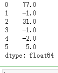

4.2.11 将等于-1的数据替换为NaN，等于-2的数据替换为0

data.replace([-1, -2], [np.nan, 0])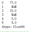

4.2.12 重命名轴索引-创建实验数据

data = DataFrame(np.arange(12).reshape((3, 4)), index=['Ohio', 'Colorado', 'New York'], columns=['one', 'two', 'three', 'four']) 

data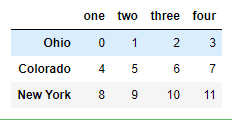

4.2.13 将标签改为大写

data.index = data.index.map(str.upper)

data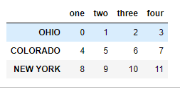

4.2.14 更换title为大写

data.rename(index=str.title, columns=str.upper)

4.2.15 修改指定的行列标签

data.rename(index={'OHIO': 'INDIANA'}, columns={'three': 'peekaboo'})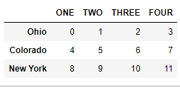

4.2.16 检测和过滤异常值-创建实验数据

np.random.seed(12345) 

data = DataFrame(np.random.randn(500, 4)) 

data.describe()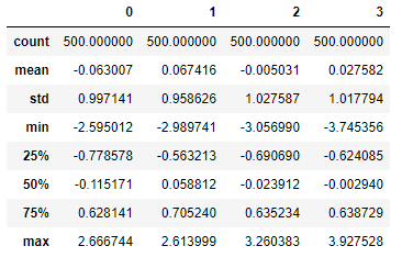

4.2.17 选出第三列绝对值大于3的

col = data[2] 

col[np.abs(col) > 3]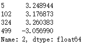

4.2.18 假设这些绝对值大于3的数据是异常值，对数据作处理

data[np.abs(data) > 3] = np.sign(data) * 3 

data.describe()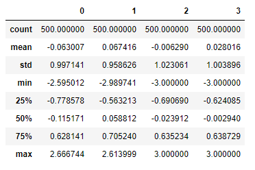

4.3 系列和DataFrame对象的绘图方法

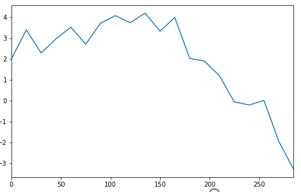
4.3.1 系列对象绘制简单的线形图

import numpy as npfrom pandas import Series,DataFrameimport matplotlib.pyplot as pltser = Series(np.random.randn(20).cumsum(), index=np.arange(0, 300, 15))ser.plot(figsize=(8,5))plt

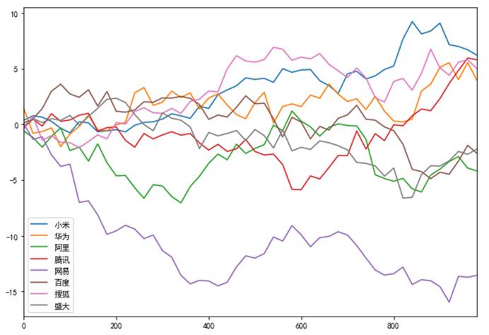
4.3.2 DataFrame对象绘制简单的线形图

import numpy as npfrom pandas import Series,DataFrameimport matplotlib.pyplot as pltfrom pylab import mplmpl.rcParams['font.sans-serif'] = ['SimHei']mpl.rcParams['axes.unicode_minus'] = Falsedf = DataFrame(np.random.randn(50, 8).cumsum(0),columns=['小米', '华为', '阿里', '腾讯','网易','百度','搜狐','盛大'],index=np.arange(0, 1000, 20))df.plot(figsize=(10,7))plt.show()

4.3.3 系列对象绘制简单的垂直和水平柱状图

import numpy as np

from pandas import Series,DataFrame

import matplotlib.pyplot as plt

fig, ax = plt.subplots(2, 1,figsize=(16,12))

data = Series(np.random.rand(10), index=list('abcdefghij'))

data.plot(kind='bar', ax=ax[0], color='r', alpha=0.5, rot=360, fontsize=16)

data.plot(kind='barh', ax=ax[1], color='b', alpha=0.7, fontsize=16)

plt.show()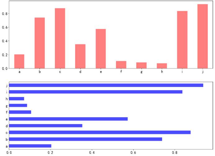

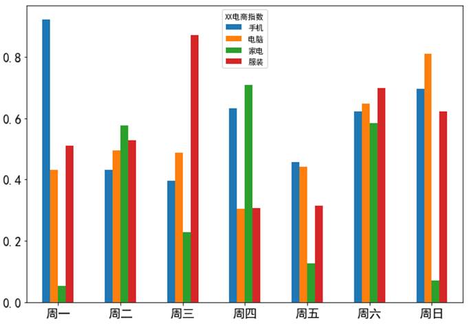
4.3.4 DataFrame对象绘制简单的垂直柱状图

import numpy as np

from pandas import Series,DataFrame

import pandas as pd

import matplotlib.pyplot as plt

from pylab import mpl

mpl.rcParams['font.sans-serif'] = ['SimHei']

mpl.rcParams['axes.unicode_minus'] = False

df = DataFrame(np.random.rand(7, 4),index=['周一', '周二', '周三', '周四', '周五', '周六', '周日'],columns=pd.Index(['手机', '电脑', '家电', '服装'], name='XX电商指数'))df.plot(kind='bar',figsize=(10,7), rot=360, fontsize=16)plt.show()

4.4 熊猫绘图函数实例

4.4.1 餐厅聚餐数据堆积柱状图

import numpy as np

from pandas import Series,DataFrame

import pandas as pd

import matplotlib.pyplot as plt

restaurant = pd.read_csv('../data/RestaurantData.csv', encoding='gbk')

num_counts = pd.crosstab(restaurant['周期'], restaurant['人数'])

num_counts = num_counts.loc[:, 2:5]

num_pcts = num_counts.div(num_counts.sum(1).astype(float), axis=0)

num_pcts.plot(kind='bar', figsize=(10,7), fontsize=16, rot=360, stacked=True)

plt.show()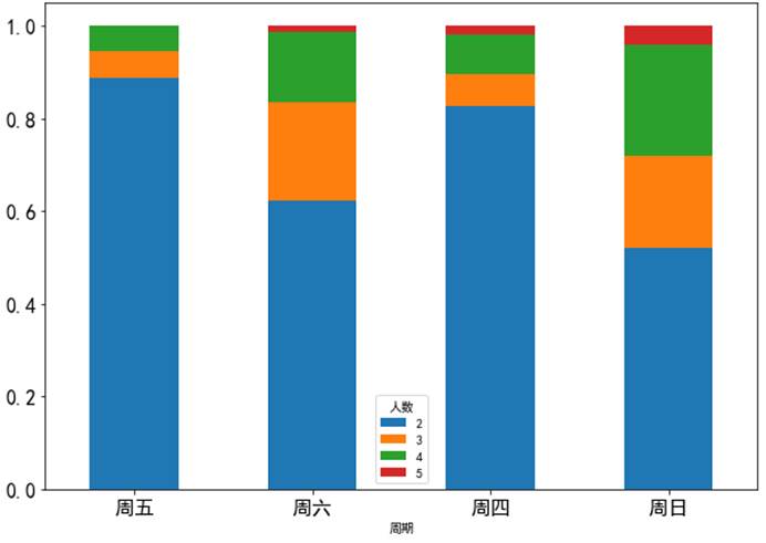

4.4.2 餐厅小费与消费总金额占比数据直方图

import numpy as np

from pandas import Series,DataFrame

import pandas as pd

import matplotlib.pyplot as plt

restaurant = pd.read_csv('../data/RestaurantData.csv', encoding='gbk')

restaurant['百分比'] = restaurant['小费'] / restaurant['消费总金额']

restaurant['百分比'].hist(bins=100, figsize=(10,7), color='r',alpha=0.7)

plt.show()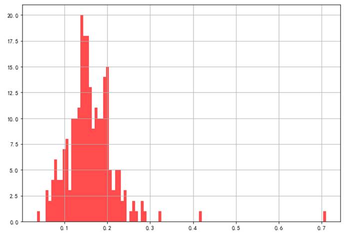

4.4.3 餐厅小费与消费总金额占比数据密度图

import numpy as np

from pandas import Series,DataFrame

import pandas as pd

import matplotlib.pyplot as plt

restaurant = pd.read_csv('../data/RestaurantData.csv', encoding='gbk')

restaurant['百分比'] = restaurant['小费'] / restaurant['消费总金额']

restaurant['百分比'].plot(kind='kde', figsize=(10,7), color='r',alpha=0.7, fontsize=16)

plt.show()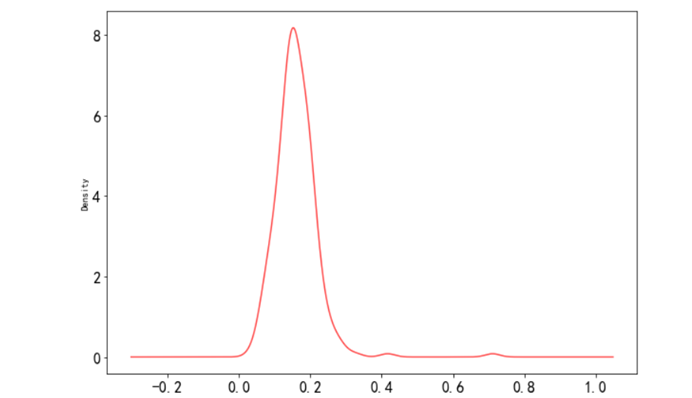

4.4.4 直方图和密度图组成双峰分布图

import numpy as np

from pandas import Series,DataFrame

import pandas as pd

import matplotlib.pyplot as plt

plt.figure(figsize=(10,7))

data1 = np.random.normal(0, 1, size=200)

data2 = np.random.normal(10, 2, size=200)

values = Series(np.concatenate([data1, data2]))

values.hist(bins=100, alpha=0.6, color='b')

values.plot(kind='kde', style='r--')

plt.show()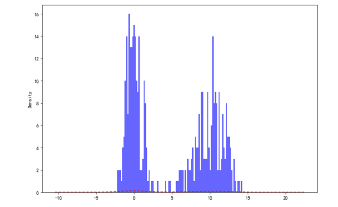

4.4.5 绘制散布图

import numpy as np

from pandas import Series,DataFrame

import pandas as pd

import matplotlib.pyplot as plt

md = pd.read_csv('../data/macrodata.csv')

data = md[['cpi', 'm1', 'tbilrate', 'unemp']]

trans_data = np.log(data).diff().dropna()

plt.figure(figsize=(10,7))

plt.scatter(trans_data['m1'], trans_data['unemp'])

plt.show()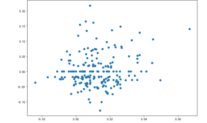

5.1 实验背景

近年来随着城市化和工业化的发展，城市空气质量越来越差，从中央到地方各级政府对城市空气质量也越发重视。并对全国各个城市的空气质量进行了长期的采样。下面对全国空气质量进行分析，可以得出我国城市空气质量的大概规律。

数据介绍

• 时间 时间
• 城市 城市
• AQI 根据细颗粒物、可吸入颗粒物、二氧化硫、二氧化氮、臭氧、一氧化碳等六项参数综合得出的空气污染程度及空气质量状况的表述。
• PM2.5 细颗粒物又称细粒、细颗粒、PM2.5。细颗粒物指环境空气中空气动力学当量直径小于等于 2.5微米的颗粒物。它能较长时间悬浮于空气中，其在空气中含量浓度越高，就代表空气污染越严重。
• PM10 总悬浮颗粒物是指漂浮在空气中的固态和液态颗粒物的总称，[1]其粒径范围约为0.1-100 微米。有些颗粒物因粒径大或颜色黑可以为肉眼所见，比可吸入颗粒物如烟尘。
• so2 二氧化硫
• no2 二氧化氮
• Co 一氧化碳
• o3 臭氧
• primary_pollutant 空气质量指数

5.2 导入支持库

5.2.1 导入支持库

import pandas as pd

import numpy as np

from pandas import Series, DataFrame

import matplotlib as mpl

import matplotlib.pyplot as plt

5.2.2 设置pandas列属性

pd.set_option('display.max_columns', None)

5.2.3 设置中文显示

mpl.rcParams["font.sans-serif"]=["SimHei"]# 用来正常显示中文标签mpl.rcParams["axes.unicode_minus"]=False# 用来正常显示负号,解决保存图像是负号'-'显示为方块的问题,或者转换负号为字符串

5.3 数据探查和处理

5.3.1 读取数据源

data = pd.read_csv('../data/air.csv')

5.3.2 简单查看数据特征

data.shape

data.columns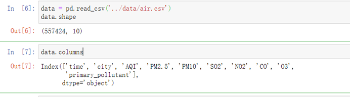

data.dtypes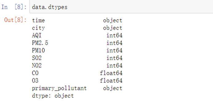

5.3.3 数据特征值初步分析

AQI_min = data.AQI.min()

AQI_max = data.AQI.max()

display(AQI_min, AQI_max)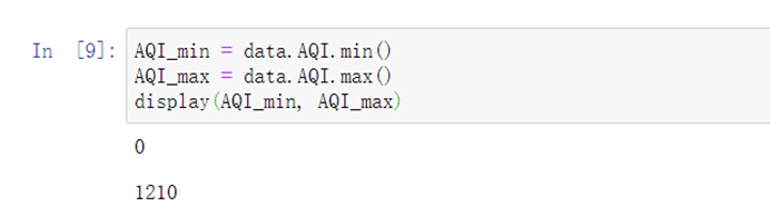

AQI_cut = pd.cut(data.AQI, bins = [AQI_min, 50, 100, 150, 200, 300, AQI_max])

AQI_count = AQI_cut.value_counts()

AQI_count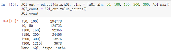

5.4 绘图简单分析

5.4.1 绘制AQI分布的柱状图

def func1():

    X = np.arange(len(AQI_count))

    Y = AQI_count

    plt.figure(figsize=(8,6))

    plt.bar(X,Y,color='steelblue',alpha=0.8)

    plt.title('AQI分布图')

    plt.xlabel('AQI区间')

    plt.ylabel('2014-2018年AQI天数')

    plt.xticks(np.arange(len(AQI_count)),AQI_count.index, rotation=30)

    plt.ylim([0,320000])

    percents = [str(round(i*100,2)) + '%'for i in AQI_count / AQI_count.sum()]

    for x,y,z in zip(X,Y,percents):

        plt.text(x-0.2,y+5000,z)

    plt.savefig('1.png')

func1()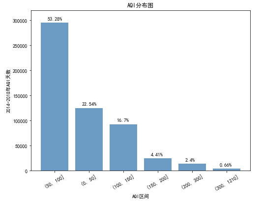

5.4.2 绘制全国污染程度饼图

# 全国污染程度饼图

def func2():

    labels = ['良(50,100]','优(0,50]','轻度污染(100,150]','中度污染(150,200]','重度污染(200,300]','严重污染(300,1210]']

    x = [i for i in AQI_count / AQI_count.sum()]

    colors= ['#32CD32','#FFDAB9','#8A2BE2','#2442aa','#dd5555','#FFFF00']

    explode = [0,0.1,0,0,0,0]   

    plt.pie(x=x,#绘图的数据

           labels=labels,#数据标签

           colors=colors,#饼图颜色

           autopct='%.1f%%',#设置百分比

           startangle=180,#设置初始角度

           #frame=1,

           #center=(2,2)

           explode=explode,#设置突出显示

           radius=2#设置饼的半径

           )

    plt.savefig('2.png')

func2()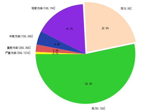

5.4.3 空气指数和pm2.5的关系

# AQI与PM2.5的关系 

def func3(pollutant,num1,num2):

    data2 = data[data[pollutant] < num1] #利用drop方法将含有特定数值的列删除

    data2 = data2[data2[pollutant] != 0]

    data2 = data2[data2['AQI'] < num2]

    data2 = data2[data2['AQI'] != 0]

    plt.scatter(data2.AQI, data2[pollutant],s=5)

    plt.xlabel('AQI')

    plt.ylabel(pollutant)

    plt.title('AQI与%s的关系' % pollutant)

    plt.savefig('%s.png' % pollutant)

func3('PM2.5',700,500)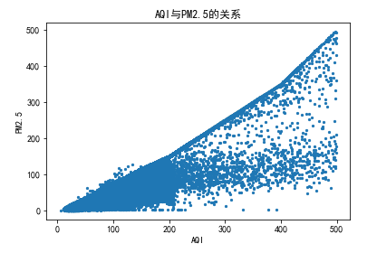

5.4.4 AQI与PM10的关系

# AQI与PM10的关系 

func3('PM10',1000,500)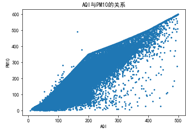

5.4.5 AQI与SO2的关系

# AQI与SO2的关系 

func3('SO2',800,500)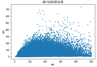

5.4.6 AQI与NO2的关系

# AQI与NO2的关系 

func3('NO2',300,500)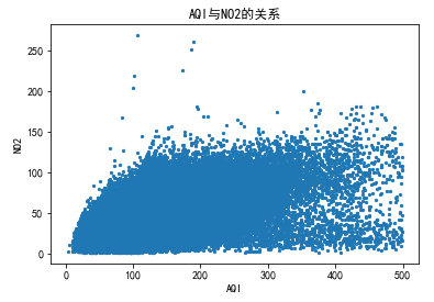

5.4.7 AQI与CO的关系

# AQI与CO的关系

func3('CO',25,500)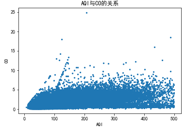

5.5 复杂绘图分析

5.5.1 全国一线及新一线AQI平均值排名

def func4():

    yixian_city = data[(data.city=='北京')|(data.city=='上海')|(data.city=='广州')|(data.city=='深圳')|(data.city=='成都')|(data.city=='杭州')|(data.city=='重庆')|(data.city=='武汉')|

                       (data.city=='苏州')|(data.city=='西安')|(data.city=='天津')|(data.city=='南京')|(data.city=='郑州')|(data.city=='长沙')|(data.city=='沈阳')|(data.city=='青岛')|

                       (data.city=='宁波')|(data.city=='东莞')|(data.city=='无锡')].groupby("city")["AQI"].mean().sort_values(ascending=False)

    plt.figure(figsize=(12,8))

    plt.barh(np.arange(len(yixian_city)), yixian_city,color='#FF0000')

    plt.yticks(np.arange(len(yixian_city)), yixian_city.index)

    plt.xlabel('AQI')

    plt.ylabel('城市')

    plt.title('全国一线城市及新一线城市AQI平均值排名')

    plt.savefig('3.png')

func4()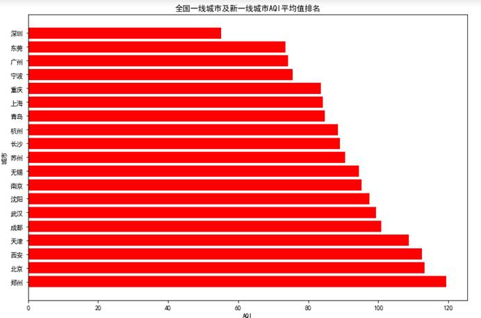

5.5.2 数据时间处理

data['year'] = pd.to_datetime(data['time']).dt.year

data['month'] = pd.to_datetime(data['time']).dt.month

data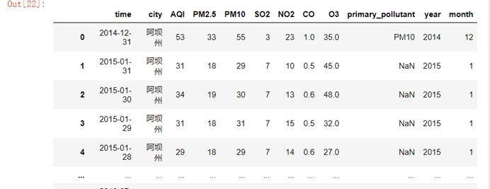

5.5.3 全国按月份污染物平均值走势

# 全国按月份污染物平均值走势

def func5():

    country_city = data.groupby('month').mean().sort_index()

    country_city2 = country_city[["AQI","PM2.5","PM10","SO2","NO2","CO"]]

    plt.figure(figsize=(12,8))

    plt.plot(country_city2,label=country_city2.columns,marker = "o" ,mec = "k" , mfc = "w" , mew = 0.5)

    plt.legend(country_city2)

    plt.xticks(np.arange(1,13))

    plt.xlim([1,12])

    plt.xlabel('月份')

    plt.ylabel('污染物')

    plt.title('全国污染物平均值走势')

    plt.savefig('4.png')

func5()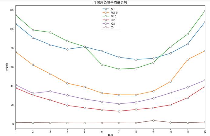

5.5.4 沿海代表城市与内地代表城市

# 沿海代表城市与内地代表城市

def func6():

    yanhai = data[(data.city=='天津')|(data.city=='深圳')|(data.city=='广州')|(data.city=='上海')].groupby("month")["AQI"].mean()

    neidi = data[(data.city=='洛阳')|(data.city=='成都')|(data.city=='西安')|(data.city=='贵阳')].groupby("month")["AQI"].mean()

    plt.figure(figsize=(12,8))

    plt.plot(yanhai,label='沿海',marker = "o" ,mec = "k" , mfc = "w" , mew = 0.5)

    plt.plot(neidi,label='内地',marker = "o" ,mec = "k" , mfc = "w" , mew = 0.5)

    plt.legend(['沿海代表城市','内地代表城市'])

    plt.xticks(np.arange(1,13))

    plt.xlim([1,12])

    plt.xlabel('月份')

    plt.ylabel('AQI平均值')

    plt.title('沿海代表城市与内地代表城市AQI平均值走势')

    plt.savefig('5.png')

func6()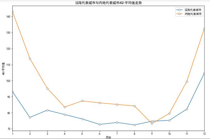

5.5.5 每年污染物柱状图

# 每年污染物柱状图

def func7_1(year):

    return [data[data.year==year]['AQI'].mean(),data[data.year==year]['PM2.5'].mean(),data[data.year==year]['PM10'].mean(),data[data.year==year]['SO2'].mean(),data[data.year==year]['NO2'].mean()]

def func7():

    plt.figure(figsize=(12,8))

    labels = ["AQI","PM2.5","PM10","SO2","NO2"]

    #设定每个柱子的宽度

    bar_width = 0.15

    x=0

    for i in [2014,2015,2016,2017,2018]:

        plt.bar(np.arange(5)+x*bar_width,func7_1(i),label=i,alpha=0.8,width=bar_width)

        x+=1

    plt.legend()

    plt.ylim([0,110])

    plt.xticks([0.295,1.295,2.295,3.295,4.295],labels)

    plt.savefig('6.png')

func7()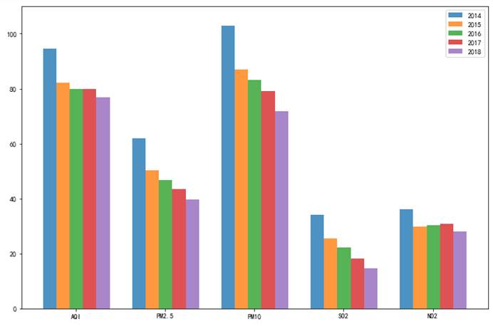

5.5.6 北京污染程度饼图

# 北京污染程度饼图

def func8(city):

    #查看不同价格区间的AQI，在当前数据集中的占比情况

    AQI_max = data[data.city==city].AQI.max()

    AQI_cut = pd.cut(data[data.city==city].AQI, bins = [0, 50, 100, 150, 200, 300, AQI_max])

    AQI_count = AQI_cut.value_counts()

    labels = ['良(50,100]','优(0,50]','轻度污染(100,150]','中度污染(150,200]','重度污染(200,300]','严重污染(300,%s]' % AQI_max]

    x = [i for i in AQI_count / AQI_count.sum()]

    colors= ['#32CD32','#FFDAB9','#8A2BE2','#2442aa','#dd5555','#FFFF00']

    explode = [0,0.1,0,0,0,0]   

    plt.pie(x=x,#绘图的数据

           labels=labels,#数据标签

           colors=colors,#饼图颜色

           autopct='%.1f%%',#设置百分比

           startangle=180,#设置初始角度

           explode=explode,#设置突出显示

           radius=1.5#设置饼的半径

           )

    plt.savefig('%s.png' % city)

func8('北京')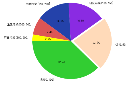

5.5.7 广州污染程度饼图

# 广州污染程度饼图

def func9():

    #查看不同价格区间的AQI，在当前数据集中的占比情况

    AQI_min = data[data.city=='广州'].AQI.min()

    AQI_max = data[data.city=='广州'].AQI.max()

    display(AQI_min, AQI_max)

    AQI_cut = pd.cut(data[data.city=='广州'].AQI, bins = [AQI_min, 50, 100, 150, 200, 207])

    AQI_count = AQI_cut.value_counts()

    labels = ['良(50,100]','优12,50]','轻度污染(100,150]','中度污染(150,200]','重度污染(200,207]']

    x = [i for i in AQI_count / AQI_count.sum()]

    colors= ['#32CD32','#FFDAB9','#8A2BE2','#2442aa','#dd5555']

    explode = [0,0.1,0,0,0]    

    plt.pie(x=x,#绘图的数据

           labels=labels,#数据标签

           colors=colors,#饼图颜色

           autopct='%.1f%%',#设置百分比

           startangle=180,#设置初始角度

           explode=explode,#设置突出显示

           radius=1.5#设置饼的半径

           )

    plt.savefig('7.png')

func9()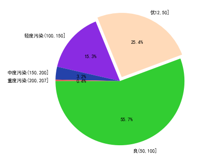

5.5.8 广州市2017年AQI走势

def func11():

    result1 = data[(data.city=='广州')&(data.year==2017)]["AQI"]

    result2 = data[(data.city=='广州')&(data.year==2017)]["time"]      

    fig = plt.figure(figsize=(12,8))

    ax = fig.add_subplot(111)#图片对象

    ax.plot(result2,result1,"-")

    ax.legend()

    ax.axis([0,144,0,400]) #画轴的范围

    month = [0,1,2,3,4,5,6,7,8,9,10,11,12]

    plt.xticks(np.arange(0,144,11.999),month) #重新设置x轴间隔和刻度值

    plt.xlabel('月份')

    plt.ylabel('AQI')

    plt.title('广州市2017年AQI走势')

    plt.savefig('9.png')

func11()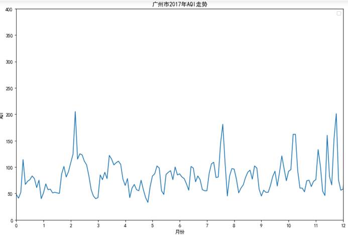

6.1 背景介绍

6.1.1 实验背景

随着房地产市场发展，房价越来越高。为了的到影响房价的增长因素，现在从数据角度出发，分析以下左右房价的因素。

数据介绍

• CATE 城区
• 卧室数量
• 大厅 客厅
• 面积 面积
• floor 地面高度，楼层
• 地铁 附近是否有地铁
• school 附近是否有学校
• 价格 价格
• 名称
• 地区区域

6.2 载入数据

6.2.1 导入支持库

import math

import numpy as np

import pandas as pd

from pandas import Series,DataFrame

import matplotlib.pyplot as plt

import statsmodels.api as sm

from scipy import stats

from statsmodels.stats.outliers_influence import summary_table

from pylab import mpl

import copy

注：若没有statsmodels模块，请到Terminal用如下命令安装

sudo pip3 install statsmodels

# Terminal在jupyter首页NEW-Other-Terminal

6.2.2 载入数据

data_source='../data/housedata.csv'#数据源文件

df = pd.read_csv(data_source,encoding='UTF8') #读入二手房数据

6.2.3 设置中文显示

plt.rcParams['font.sans-serif']=['SimHei'] #用来正常显示中文标签

plt.rcParams['axes.unicode_minus']=False #用来正常显示负号

6.3 数据探查

6.3.1 查看数据源数据特征

df_ana = df

df_ana.head() # 样本取样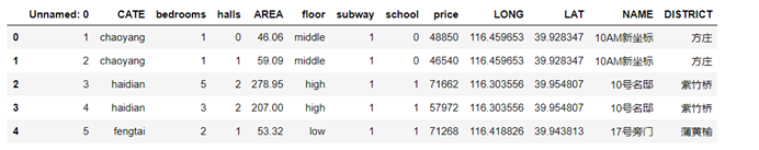

6.3.2 继续检查样本数量

len(df_ana) # 样本数量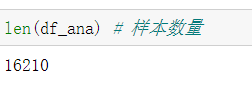

6.3.3 将价格单位转化为万元

df_ana['price'] = df_ana['price']/10000

df_ana.head()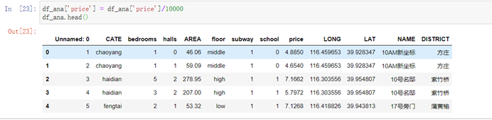

6.3.4 将CATE（城区）列转化为中文

list_roma = list(set(df_ana['CATE']))

list_roma.sort()

list_roma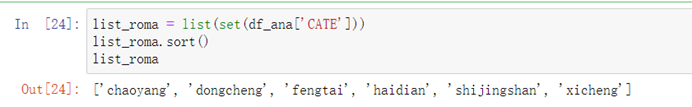

list_chinese = ['朝阳','东城','丰台','海淀','石景山','西城']

dict_map = dict()

for i in range(0,len(list_roma)):

    dict_map[list_roma[i]]=list_chinese[i]

dict_map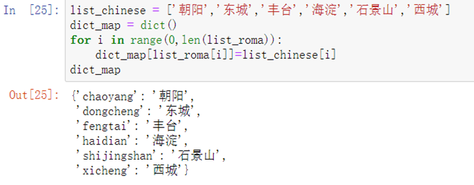

用汉字替换拼音：

for x in dict_map.keys():

    df_ana['CATE'] = df_ana['CATE'].str.replace(x,dict_map[x])

df_ana.head()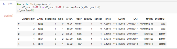

6.3.5 调整城区和楼层的因子水平顺序

df_ana = df_ana.sort_values(by = ['floor'],axis = 0,ascending = True)

df_ana.head()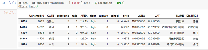

6.4 简单绘图分析

6.4.1 分析数据源，绘制因变量直方图

plt.hist(df_ana["price"],color='lightblue')

plt.xlabel('单位面积房价(万元/平方米)')

plt.ylabel('频度')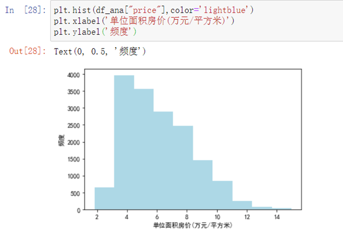

6.4.2 检查售价均值

df_price_avg = df_ana['price'].mean()

df_price_avg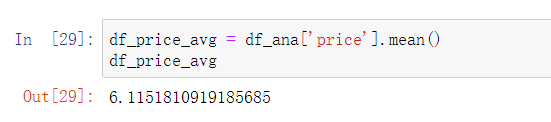

6.4.3 检查中位数

df_price_middle = df_ana['price'].median()

df_price_middle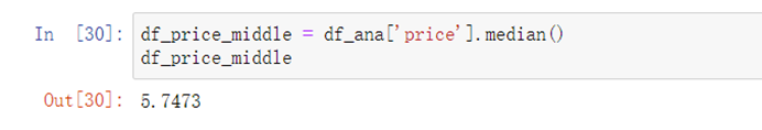

6.4.4 检查最大值

df_price_max = df_ana.sort_values(by='price',ascending=False).head(1)

df_price_max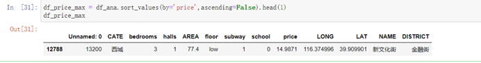

6.4.5 检查最小值

df_price_min = df_ana.sort_values(by='price',ascending=True).head(1)

df_price_min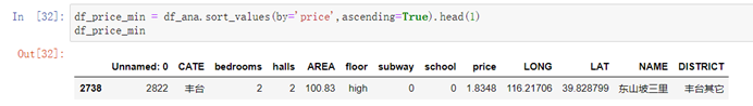

6.4.6 绘制房价的分组箱线图

df_ana.boxplot(column=["price"],by=['CATE'])

plt.ylabel("单位面积房价(万元/平方米)")

plt.xlabel("城区")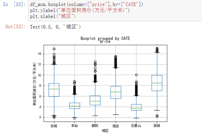

6.4.7 地铁、学区的分组箱线图

df_ana.boxplot(column=['price'],by=['subway'],labels=['非地铁房','地铁房'])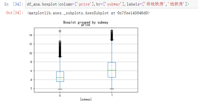

df_ana.boxplot(column=['price'],by=['school'],labels=['非学区房','学区房'])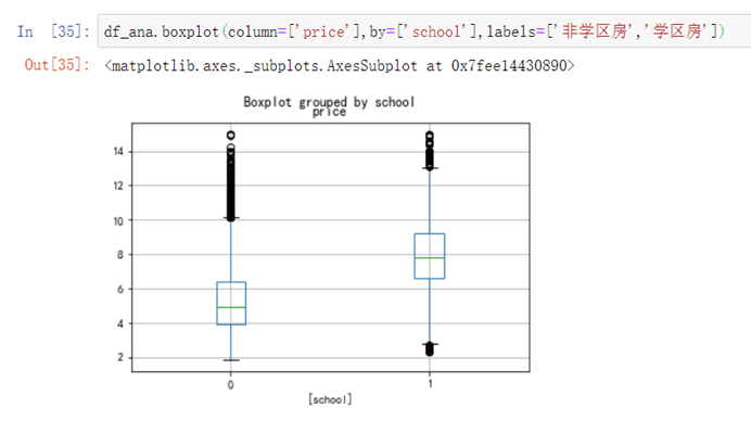

6.4.8 考察房源，客厅、卧室和楼层是否对价格有影响

df_ana.boxplot(column=['price'],by=['bedrooms'])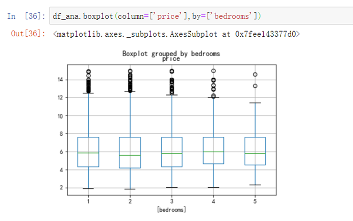

考察客厅数量对房价的影响：

df_ana.boxplot(column=['price'],by=['halls'])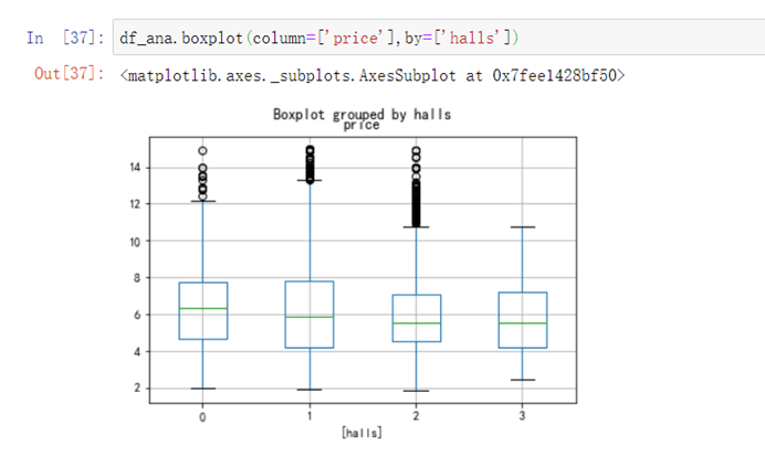

考察楼层高低对房价的影响：

df_ana.boxplot(column=['price'],by=['floor'])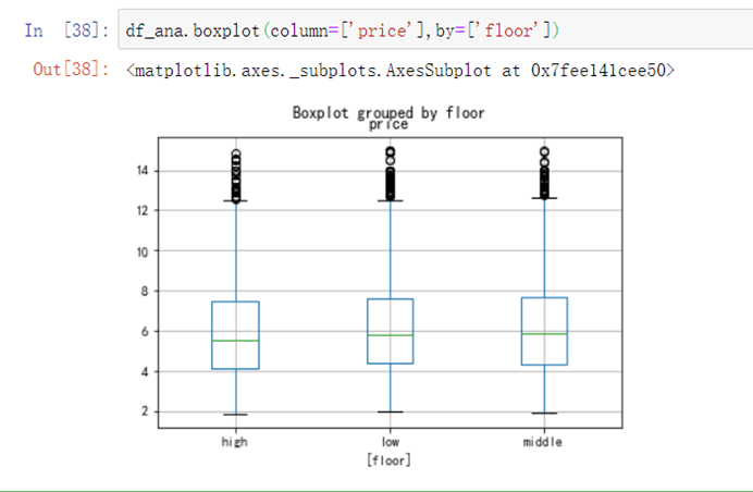

6.4.9 考察房屋面积和单位价格的关系

plt.plot(df_ana['AREA'],df_ana['price'],'ro',color='lightblue')

plt.xlabel('面积(平方米)')

plt.ylabel('单位面积房价(万元/平方米)')

plt.show()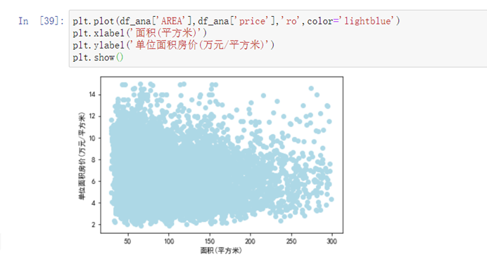

6.4.10 建立线性回归模型

客厅数做因子化处理，变成二分变量，使得建模有更好的解读。

def fun(x):

    if isinstance(x,int): 

        if x == 0:

            return 0

        else:

            return 1

    else:

        return 0

style_halls = df_ana

df_ana['have_halls'] = df_ana['halls'].apply(lambda x: fun(x))

col_n =['CATE','bedrooms','AREA','floor','subway','school','have_halls']

将变量参数数据化

y=df_ana.price

x=pd.DataFrame(df_ana,columns=col_n)  #设置自变量x

x_dum_cate=pd.get_dummies(x['CATE'])  #对哑变量编码

x_dum_floor=pd.get_dummies(x['floor'])  #对哑变量编码

del x['CATE']

del x['floor']

x=pd.concat([x,x_dum_cate],axis=1)

x=pd.concat([x,x_dum_floor],axis=1)

X=sm.add_constant(x)  #增加截距项

查看数据：

X.head()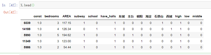

线性回归模型（因变量：单位面积房价）：

model=sm.OLS(y,X)

result=model.fit()

result.params  #显示回归系数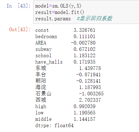

result.summary()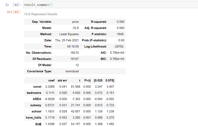

y_hat=result.predict(X)

residuals=y-y_hat

fig = plt.figure()

6.4.11 验证模型是否符合线性模型

fg1 = fig.add_subplot(221)

fg1.set_title('Residuals VS Fitted') 

plt.xlabel('Fitted Values')

plt.ylabel('Residuals')

plt.scatter(y_hat,residuals)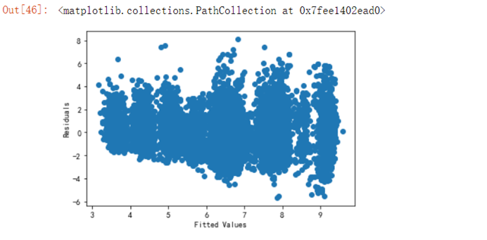

6.4.12 验证房价是否是正太分布

residuals_n=(residuals-np.mean(residuals))/np.std(residuals)

sorted_=np.sort(residuals_n)

yvals=np.arange(len(sorted_))/float(len(sorted_))

x_label=stats.norm.ppf(yvals)

fg2 = fig.add_subplot(222)

fg2.set_title('Normal Q-Q') 

plt.xlabel('Theoretical Quantiles')

plt.ylabel('Standardized residuals')

plt.scatter(x_label,sorted_)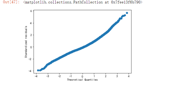

6.5 复杂绘图分析

6.5.1 换一种方法重新验证模型是否符合线性模型

residuals_sq=np.sqrt(abs(residuals_n))

fg3 = fig.add_subplot(223)

fg3.set_title('Scale-Location') 

plt.xlabel('Fitted Values')

plt.ylabel('sqrt(Standardized residuals)')

plt.scatter(y_hat,residuals_sq)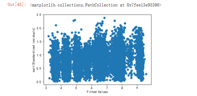

6.5.2 考察样本异常值

n=len(y)

y_m=np.mean(y)

Lyy=np.sum((y-y_m)**2)

Hii=1/n+(y-y_m)**2/Lyy

fg4 = fig.add_subplot(224)  #绘制每个点的库克距离，检测异常点用

fg4.set_title("Cook's distance") 

plt.xlabel('Obs number')

plt.ylabel("Cook's distance")

plt.plot(Hii.tolist())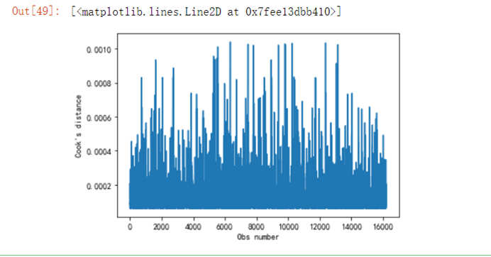

6.5.3 取对数后重新做以上验证

#对房价取对数，得到——y_log

y_log=df_ana['price'].apply(lambda x:math.log(x))

#对数房价回归模型

model=sm.OLS(y_log,X)

result=model.fit()

result.params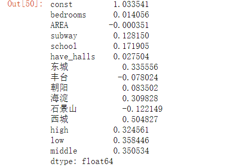

考察模型参数：

result.summary()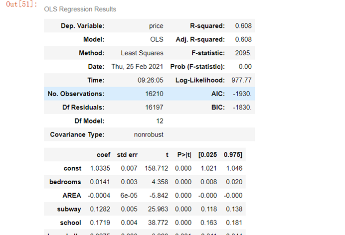

6.5.4 建立新的交叉对数模型

X2=copy.deepcopy(X)

X2['丰台_学区']=X2['丰台']*X2['school']

X2['朝阳_学区']=X2['朝阳']*X2['school']

X2['东城_学区']=X2['东城']*X2['school']

X2['海淀_学区']=X2['海淀']*X2['school']

X2['石景山_学区']=X2['石景山']*X2['school']

X2['西城_学区']=X2['西城']*X2['school']

#对数房价、城区/学区交叉项回归模型

model=sm.OLS(y_log,X2)

result=model.fit()

residus=result.resid

result.params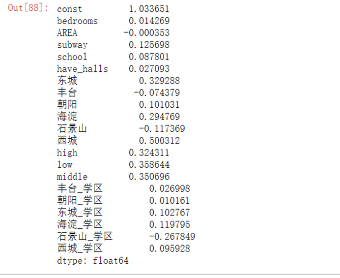

6.5.5 验证交叉对数模型是否正确

fg = fig.add_subplot(221)

fg.set_title('Residuals VS Fitted') 

plt.xlabel('Fitted Values')

plt.ylabel('Residuals')

plt.scatter(y_hat,residuals)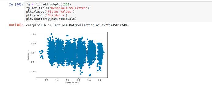

6.5.6 验证房价是否是正太分布

residuals_n=(residuals-np.mean(residuals))/np.std(residuals)

sorted_=np.sort(residuals_n)

yvals=np.arange(len(sorted_))/float(len(sorted_))

x_label=stats.norm.ppf(yvals)

fg = fig.add_subplot(222)

fg.set_title('Normal Q-Q') 

plt.xlabel('Theoretical Quantiles')

plt.ylabel('Standardized residuals')

plt.scatter(x_label,sorted_)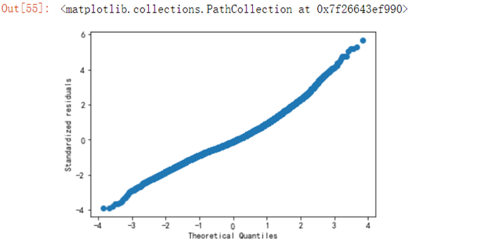

6.5.7 取平方根，除去符号影响重新验证模型是否符合线性模型

residuals_sq=np.sqrt(abs(residuals_n))

fg3 = fig.add_subplot(223)

fg3.set_title('Scale-Location') 

plt.xlabel('Fitted Values')

plt.ylabel('sqrt(Standardized residuals)')

plt.scatter(y_hat,residuals_sq)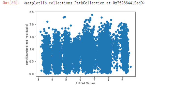

n=len(y)

y_m=np.mean(y)

Lyy=np.sum((y-y_m)**2)

Hii=1/n+(y-y_m)**2/Lyy

fg4 = fig.add_subplot(224)  #绘制每个点的库克距离，检测异常点用

fg4.set_title("Cook's distance") 

plt.xlabel('Obs number')

plt.ylabel("Cook's distance")

plt.plot(Hii.tolist())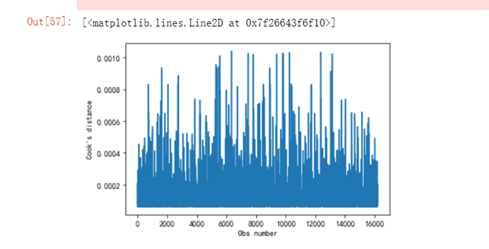

假设需要在西城区买一套临近地铁的学区房，面积85平米。大概需要多少钱。

house_new=[1,2,85,1,1,1,0,0,0,0,0,1,0,1,0,0,0,0,0,0,1]

price_new=np.exp(result.predict(house_new))

#单价

price_new

print('房价预测值为：%.2f'%price_new,'万元/平方米')

print('房价预测值为：%.2f'%(85*price_new),'万元')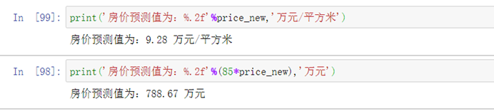

7.1 背景介绍

7.1.1实验背景

电影娱乐产业越发发达，投资商希望能从电影的各种数据中找到最可能赚钱的电影有什么特点。

数据介绍

• 预算 预算 预算
• 流派 电影名数据
• 首页 网站主页
• 编号
• 关键字 关键字
• original_language 语言
• original_title 标题
• 概述 概述
• 人气 人气
• 人气 电影商
• production_countries 电影商拍摄地
• release_date 发布日期
• 收入 收入
• runtime 电影时长
• spoken_languages 电影语言
• 状态 状态
• 状态 标语
• 标题 标题
• vote_average 评分
• 评分人数
• movie_id 电影 id
• 标题 标题
• cast 投票人信息
• 船员 所有信息

7.2 载入数据

7.2.1 导入支持库

import pandas as pd

import numpy as np

import matplotlib.pyplot as plt

import json

7.2.3 设置中文标签显示

plt.rcParams['font.sans-serif']=['SimHei'] #用来正常显示中文标签

plt.rcParams['axes.unicode_minus']=False #用来正常显示负号

7.2.4 载入数据集

movies=pd.read_csv(r'../data/tmdb_5000_movies.csv',sep=',')

credit=pd.read_csv(r'../data/tmdb_5000_credits.csv',sep=',')

7.3 数据清洗

7.3.1 检查两个id列和title列是否真的相同

(movies['id']==credit['movie_id']).describe()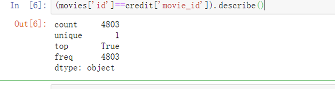

(movies['title']==credit['title']).describe()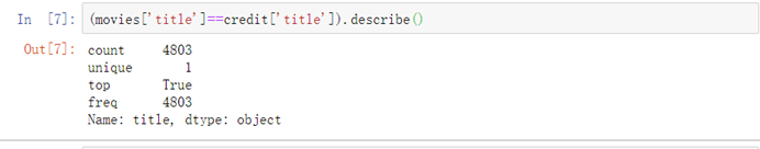

7.3.2 删除多余列

del credit['movie_id']

del credit['title']

del movies['homepage']

del movies['spoken_languages']

del movies['original_language']

del movies['original_title']

del movies['overview']

del movies['tagline']

del movies['status']

7.3.3 合并两个数据集

full_df=pd.concat([credit,movies],axis=1)#横向连接

7.3.4 处理缺失值-首先找到缺失值

nan_x=full_df['runtime'].isnull()

full_df.loc[nan_x,:]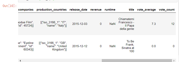

7.3.5 处理缺失值

full_df.loc[2656,'runtime']=98

full_df.loc[4140,'runtime']=82

7.3.6 查找release_data的缺失值

nan_y=full_df['release_date'].isnull()

full_df.loc[nan_y,:]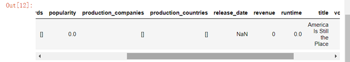

7.3.7 处理release_data的缺失值

full_df.loc[4553,'release_date']='2014-06-01'

7.3.8 将release_date的类型转换成日期类型

full_df['release_date']=pd.to_datetime(full_df['release_date'],errors='coerce',format='%Y-%m-%d')

full_df.info()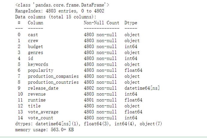

7.3.9 转换成日期格式后，提取对应的年份

full_df['release_year']=full_df['release_date'].map(lambda x : x.year)

full_df.loc[:,'release_year'].head()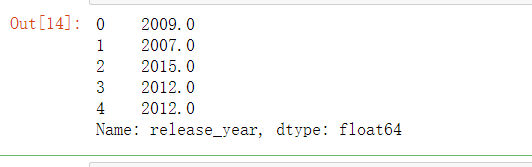

7.3.10 处理json格式类型-提取json格式，使用json.loads将json格式转化成字符串

json_cols=['genres','keywords','production_companies','production_countries','cast','crew']

for i in json_cols:

    full_df[i]=full_df[i].apply(json.loads)

def get_names(x):

    return ','.join(i['name'] for i in x)

full_df['genres']=full_df['genres'].apply(get_names)

full_df['keywords']=full_df['keywords'].apply(get_names)

full_df['production_companies']=full_df['production_companies'].apply(get_names)

full_df['production_countries']=full_df['production_countries'].apply(get_names)

full_df['genres'].head()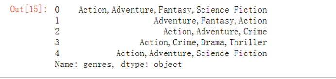

7.3.11 获取所有电影类型

real_genres=set()

for i in full_df['genres'].str.split(','):

    real_genres=real_genres.union(i)

real_genres=list(real_genres)#将集合转换成列表

real_genres.remove('')#删除空格

print(real_genres)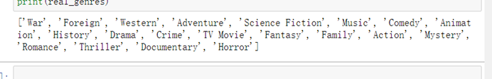

7.3.12 将所有类型添加到列表

for i in real_genres:

  full_df[i]=full_df['genres'].str.contains(i).apply(lambda x:1 if x else 0)

full_df.head(2)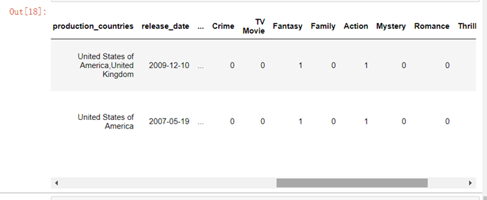

7.3.13 获取年份和类型子集,按年分组统计每年各类型电影数量

part1_df=full_df[['release_year', 'Family', 'War', 'Documentary', 'Mystery', 'Foreign','Science Fiction', 'History', 'Adventure', 'Music', 'Animation',

       'Western', 'Action', 'Crime', 'Comedy', 'Drama', 'Romance', 'Horror','Thriller', 'Fantasy', 'TV Movie']]

year_cnt=part1_df.groupby('release_year').sum()

year_cnt.tail()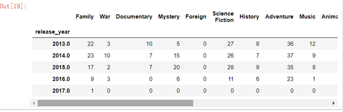

7.3.14 每年电影类别数量

plt.figure(figsize=(10,6))

plt.rc('font',family='SimHei',size=10)#设置字体和大小，否则中文无法显示

ax1=plt.subplot(1,1,1)

year_cnt.plot(kind='line',ax=ax1)

plt.title('每年电影类型数量')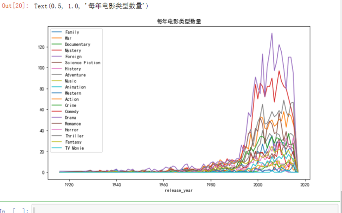

7.3.15 不同电影类型总数量

genre=year_cnt.sum(axis=0)#对列求和

genre=genre.sort_values(ascending=True)

genre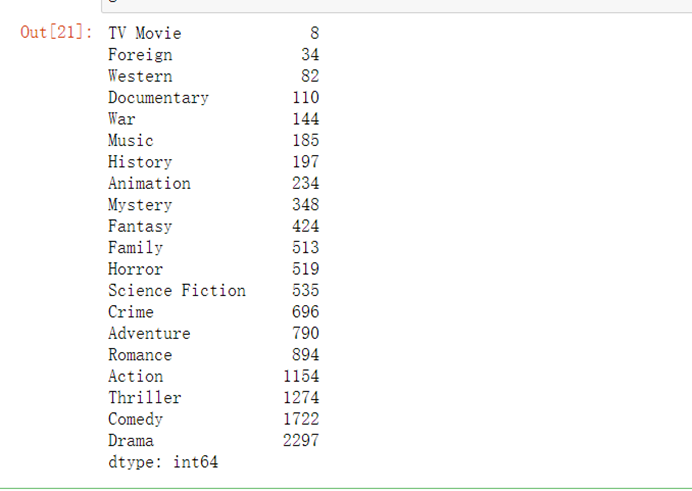

7.4 简单绘图分析

7.4.1 绘制分类数据横向条形图

plt.figure(figsize=(10,6))

plt.rc('font',family='STXihei',size=10.5)

ax2=plt.subplot(1,1,1)

label=list(genre.index)

data=genre.values

rect=ax2.barh(range(len(label)),data,color='#03A2FF',alpha=1)

ax2.set_title('不同电影类型数量')#设置标题

ax2.set_yticks(range(len(label)))

ax2.set_yticklabels(label)

#添加数据标签

for x,y in zip(data,range(len(label))):

    ax2.text(x,y,'{}'.format(x),ha='left',va='center')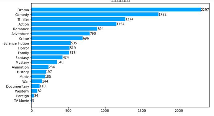

7.4.2 计算不同类型电影收入(亿元)

r={}

for i in real_genres:

    r[i]=full_df.loc[full_df[i]==1,'revenue'].sum(axis=0)/100000000

revenue=pd.Series(r).sort_values(ascending=True)

revenue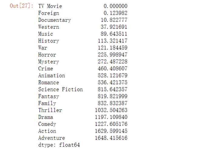

7.4.3 绘制电影收入的横向条形图

plt.figure(figsize=(12,6))

plt.rc('font',family='Simhei',size=10.5)

ax=plt.subplot(1,1,1)

label=revenue.index

data=revenue.values

ax.barh(range(len(label)),data,color='#03A2FF',alpha=1)

ax.set_yticks(range(len(label)))#设置y轴刻度

ax.set_yticklabels(label)#设置刻度名称

ax.set_title('不同类型电影收入')

#添加数据标签

for x,y in zip(data,range(len(label))):

    ax.text(x,y,'{:.1f}'.format(x))#坐标位置，及要显示的文字内容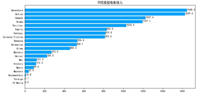

7.4.4 票房收入影响因素分析

corr=full_df.corr()#计算各变量间的相关系数矩阵

corr_revenue=corr['revenue'].sort_values(ascending=False)#提取收入与其他变量间的相关系数，并从大到小排序

corr_revenue.head(10)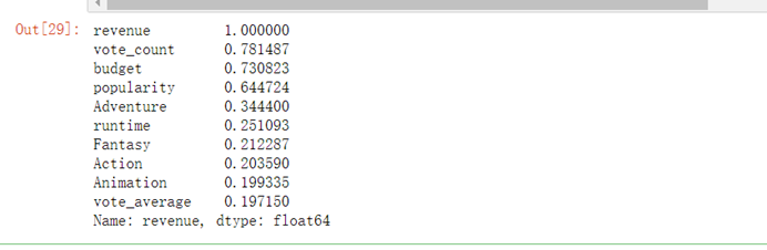

7.4.5 绘制散点图，分析预算与revenue的相关性

x=full_df.loc[:,'budget']

y=full_df.loc[:,'revenue']

plt.rc('font',family='SimHei',size=10.5)

plt.scatter(x,y,color='#03A2FF')

plt.xlabel('budget')

plt.ylabel('revenue')

plt.title('budget与revenue的散点图')

plt.show()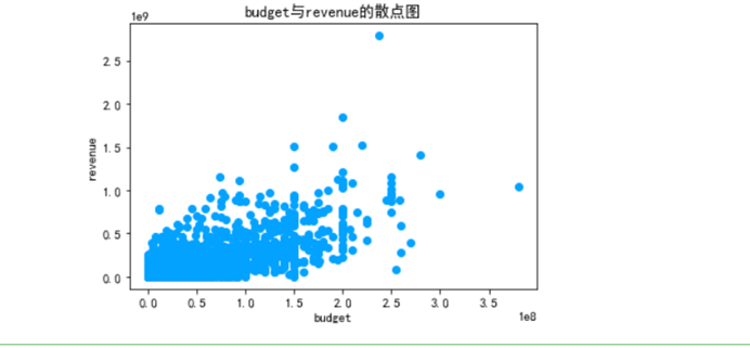

7.4.6 原创电影与改编电影分析

part2_df=full_df.loc[:,['release_year','keywords']]

part2_df['based_on_novel']=part2_df['keywords'].str.contains('based on novel').apply(lambda x:1 if x else 0)  

part2_df['not_based_on_novel']=part2_df['keywords'].str.contains('based on novel').apply(lambda x:0 if x else 1)  

part2_df.head()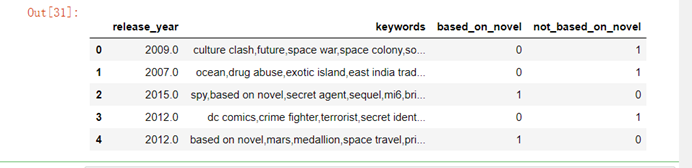

novel_per_year=part2_df.groupby('release_year')['based_on_novel','not_based_on_novel'].sum()

novel_per_year.tail()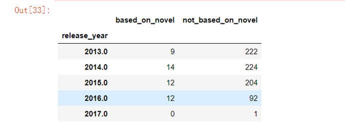

7.4.7 绘制原创电影与改变电影趋势图

novel_per_year.plot()

plt.rc('font',family='SimHei',size=10.5)

plt.title('原创电影与改编电影数量趋势图')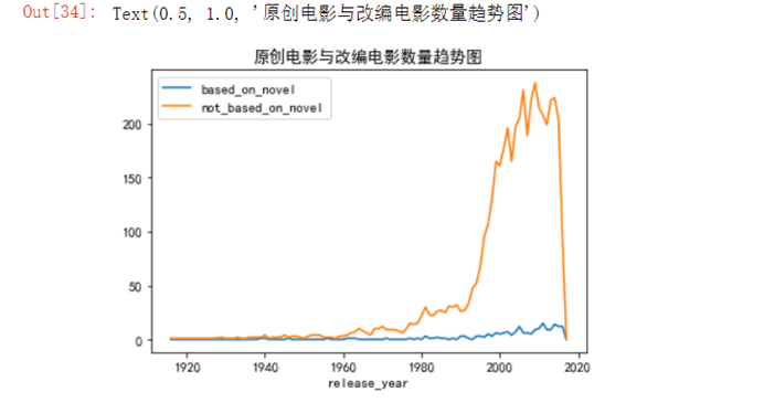

7.4.8 原创电影与改编电影总数

novel_all=[part2_df['based_on_novel'].sum(axis=0),part2_df['not_based_on_novel'].sum(axis=0)]

novel_rate=novel_all/sum(novel_all)

novel_rate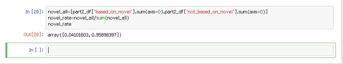

7.4.9 绘制原创电影和改编电影比例饼图

plt.figure(figsize=(6,6))

plt.rc('font',family='SimHei',size=10.5)

ax=plt.subplot(111)#与plt.sumplot(1,1,1)效果一样

labels=['based_on_novel','not_based_on_novel']

colors=['#03A2FF','#0AAA99']

ax.pie(novel_rate,labels=labels,colors=colors,startangle=90,autopct='%1.1f%%')

ax.set_title('原创电影与改编电影数量占比')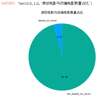

7.5 复杂绘图分析

分析电影主题关进词

7.5.1 获取所有关键词及其对应词频

keywords_dic={}

def get_keywords(x):

    for i in x:

        keywords_dic[i]=keywords_dic.get(i,0)+1

    return keywords_dic[i]     

keywords = full_df['keywords'].str.split(',').apply(get_keywords)

keywords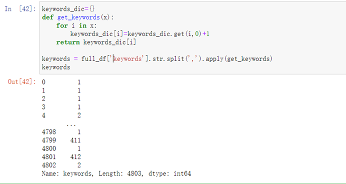

7.5.2 绘制词云图

安装wordcloud安装包：!pip install wordcloud

import matplotlib.pyplot as plt

from wordcloud import WordCloud,STOPWORDS

import pandas as pd

wordcloud=WordCloud(max_words=500 #最大词数

#                    ,font_path="DejaVuSerif.ttf" 

#自定义字体

                    ,background_color="white" #背景颜色

                    ,max_font_size=80 #最大字号

                    ,prefer_horizontal=100 #词语水平方向排版出现的频率，设置为100表示全部水平显示

                    ,stopwords=STOPWORDS #使用屏蔽词

                    )

wordcloud=wordcloud.fit_words(keywords_dic)

plt.imshow(wordcloud)

plt.axis('off')

plt.show()

wordcloud.to_file('worldcloudt.jpg')

7.5.3 统计各个国家的电影数

part3_df=full_df[['production_countries','id','release_year']]#提取需要的列子集

#由于有的电影产地属于多个国家，故需要对production_countries进行分列

split_df=pd.DataFrame([x.split(',') for x in part3_df['production_countries']],index=part3_df.index)

#将分列后的数据集与源数据集合并

part3_df=pd.merge(part3_df,split_df,left_index=True,right_index=True)

#下面代码实现列转行

st_df=part3_df[['release_year',0,1,2,3]]

st_df=st_df.set_index('release_year')

st_df=st_df.stack()

st_df=st_df.reset_index()

st_df=st_df.rename(columns={0:'production_countries'})#对列重命名

countries=st_df['production_countries'].value_counts()#统计各个国家的电影数

countries.sum()

countries_rate=countries/countries.sum()#计算占比

countries_top5=countries_rate.head(5)

other={'other':1-countries_top5.sum()}

countries_top6=countries_top5.append(pd.Series(other))

countries_top6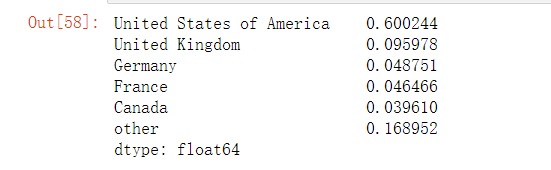

7.5.4 绘制安国家分类的电音出品饼图

labels=list(countries_top6.index)

plt.figure(figsize=(6,6))

plt.rc('font',family='SimHei',size=10.5)

ax=plt.subplot(1,1,1)

ax.pie(countries_top6,labels=labels,startangle=90,autopct='%1.1f%%')

ax.set_title('电影产地分布')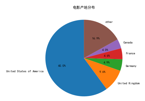

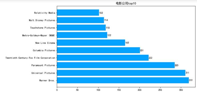
7.5.5 统计各个电影公司电影数

part4_df=full_df[['production_companies','release_year']]

split_df=pd.DataFrame([x.split(',') for x in part4_df['production_companies']],index=part4_df.index)

part4_df=pd.merge(part4_df,split_df,left_index=True,right_index=True)

del part4_df['production_companies']

part4_df=part4_df.set_index('release_year')

part4_df=part4_df.stack()

part4_df=part4_df.reset_index()

part4_df=part4_df.rename(columns={0:'production_companies'})

companies=part4_df['production_companies'].value_counts()

companies_top10=companies[companies.index!=''].head(10)

companies_top10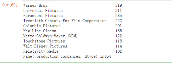

7.5.6 绘制电影公司条形图

plt.figure(figsize=(10,6))

plt.rc('font',family='SimHei',size=10.5)

ax=plt.subplot(111)

ax.barh(range(10),companies_top10.values,color='#03A2FF')

ax.set_title('电影公司top10')

ax.set_yticks(range(10))

ax.set_yticklabels(companies_top10.index)

for x,y in zip(companies_top10.values,range(10)):

    ax.text(x,y,'{}'.format(x),ha='left',va='center')