基于LSTM+前向均值滤波后处理的癫痫发作检测(包含数据集)

引言

癫痫是一种常见的神经系统疾病，患者会经历反复的癫痫发作。早期检测和预警对于改善患者的生活质量至关重要。近年来，深度学习技术，尤其是长短期记忆网络（LSTM），在时间序列数据分析中表现出色，被广泛应用于癫痫发作检测任务。本文将介绍如何使用LSTM构建一个癫痫发作检测模型。

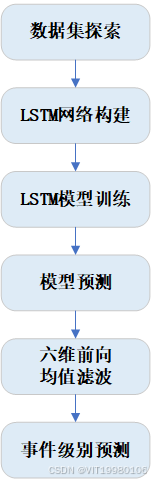
整体框架

数据集探索

癫痫数据集来源于真实的癫痫患者，通过手环记录患者的加速度和角速度，本次实验是提取特征后的加速度角速度特征集合，数据集的时间单位为秒，对应的标签事件维度也是秒级别的。

import matplotlib.pyplot as plt
from scipy.io import loadmat

# 定义路径
train_data_path = "lstm_data_training.mat"  # 替换为你的训练数据路径
test_data_path = "lstm_data_test.mat"  # 替换为你的测试数据路径

# 计算标签分布
def cal_label(data_path):
    data = loadmat(data_path)
    label_list = data["lstm_lab"][:, 0]  # 获取标签列
    count_0 = sum(label_list == 0)  # 计算标签为0的数量
    count_1 = sum(label_list == 1)  # 计算标签为1的数量
    return count_0, count_1

# 绘制标签分布
def plot_label_distribution(train_data_path, test_data_path):
    # 获取训练集和测试集的标签分布
    count_0_train, count_1_train = cal_label(train_data_path)
    count_0_test, count_1_test = cal_label(test_data_path)

    # 创建子图，调整布局
    fig, ax = plt.subplots(1, 2, figsize=(14, 7))

    # 绘制训练数据集标签分布
    ax[0].bar(['0', '1'], [count_0_train, count_1_train], color=['skyblue', 'lightcoral'])
    ax[0].set_title('Training Dataset Label Distribution', fontsize=14)
    ax[0].set_xlabel('Label', fontsize=12)
    ax[0].set_ylabel('Count', fontsize=12)
    ax[0].text(0, count_0_train + 0.1, f'0: {count_0_train}', ha='center', fontsize=12)
    ax[0].text(1, count_1_train + 0.1, f'1: {count_1_train}', ha='center', fontsize=12)

    # 绘制测试数据集标签分布
    ax[1].bar(['0', '1'], [count_0_test, count_1_test], color=['skyblue', 'lightcoral'])
    ax[1].set_title('Test Dataset Label Distribution', fontsize=14)
    ax[1].set_xlabel('Label', fontsize=12)
    ax[1].set_ylabel('Count', fontsize=12)
    ax[1].text(0, count_0_test + 0.1, f'0: {count_0_test}', ha='center', fontsize=12)
    ax[1].text(1, count_1_test + 0.1, f'1: {count_1_test}', ha='center', fontsize=12)

    plt.tight_layout()
    plt.show()

# 调用绘制函数
plot_label_distribution(train_data_path, test_data_path)

癫痫病数据集是患者真实的手坏秒级数据，因此负样本数量叫少。

LSTM网络构建

使用tensorflow实现LSTM网络，具体代码如下。

# 定义 LSTM 模型
def build_lstm_model(input_shape, n_class):
    model = Sequential()
    model.add(LSTM(100, return_sequences=True, input_shape=input_shape, name="lstm1"))
    model.add(Dropout(0.2))
    model.add(LSTM(50, return_sequences=False, name="lstm2"))
    model.add(Dense(n_class, activation="softmax", name="classifier"))
    model.compile(
        loss="categorical_crossentropy", optimizer=Adam(learning_rate=1e-3), metrics=["accuracy"]
    )
    model.summary()
    return model

LSTM网络训练

# 主训练函数
def train_model(train_data_path, save_path, n_epoch=10, batch_size=32):
    # 加载训练数据
    print("加载训练数据...")
    data = loadmat(train_data_path)
    x_train = data["lstm_data"]  # 输入数据
    y_train = data["lstm_lab"][:, 0]  # 取第一列作为发作标签（0 或 1）

    # 将标签转换为 one-hot 编码
    y_train = to_categorical(y_train, num_classes=2)

    # 确定输入形状
    input_shape = (x_train.shape[1], x_train.shape[2])  # (时间步长, 特征数)
    n_class = y_train.shape[1]  # 类别数

    # 构建模型
    model = build_lstm_model(input_shape, n_class)

    # 定义早停
    early_stop = EarlyStopping(
         monitor="val_loss", patience=5, restore_best_weights=True, verbose=1
    )

    # 开始训练
    print("开始训练...")
    history = model.fit(
        x_train,
        y_train,
        epochs=n_epoch,
        batch_size=batch_size,
        validation_split=0.2,
        callbacks=[early_stop],
        verbose=1,
    )

    # 保存模型
    model_file = os.path.join(save_path, "best_model.keras")
    model.save(model_file)
    print(f"训练完成，模型已保存到: {model_file}")

    return model_file

LSTM预测

 # 加载测试数据
    data = loadmat(test_data_path)
    x_test = data["lstm_data"]
    lstm_lab = data["lstm_lab"]
    y_true = lstm_lab[:, 0]  # 真实标签
    print(y_true)

    # 加载模型并预测
    model = load_model(model_path)
    probabilities = model.predict(x_test)

LSTM的预测也是秒级别的

六维前向均值滤波

为了与真实的癫痫发作事件对应，通过六维的前向均值滤波对预测结果进行后处理，然后对结果进行滑动窗口处理，当预测发作概率的大于9秒时，判断为癫痫发作事件，经过与真实的癫痫发作事件对比，LSTM准确识别了所有的癫痫发作事件，且发作时间基本吻合，验证了深度学习在癫痫识别的准确性。

def count_segments(arr, threshold=0.5, length=9):
    count = 0
    consecutive = 0

    for value in arr:
        if value > threshold:
            consecutive += 1
            if consecutive == length:
                count += 1
                consecutive -= 1
        else:
            consecutive = 0

    return count


# 前向均值滤波函数
def forward_mean_filter(data, k=6):
    filtered_data = data.copy()  # 复制原始数据
    for t in range(k, len(data)):
        filtered_data[t] = np.mean(data[t - k:t])  # 用前k个点的均值替代当前点
    return filtered_data