Python的rasterio库
前言
遥感数据是通过卫星、无人机等设备获取的地球表面信息,广泛应用于农业、环境监测、城市规划等领域。处理这些数据常常需要对栅格图像进行分析,而Python的rasterio库正是解决这一需求的利器。本篇文章将带你深入了解rasterio库,帮助你掌握遥感数据处理的技巧与最佳实践。
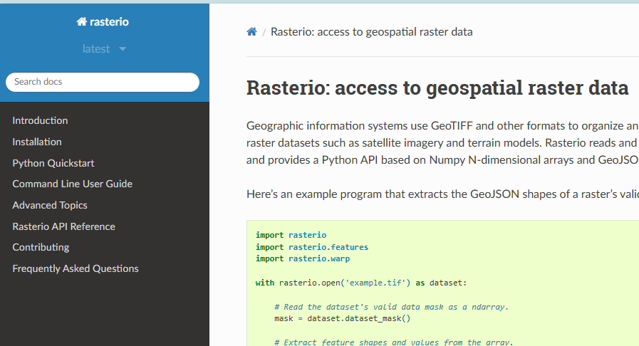
rasterio官方文档:https://rasterio.readthedocs.io/en/latest/index.html
一、rasterio库简介
rasterio是基于GDAL的Python接口封装,相比直接使用GDAL,rasterio具有以下优势:
✅ 更简洁的API设计
✅ 原生支持NumPy数组操作
✅ 完美集成Python科学计算生态
✅ 支持多线程读写加速
典型应用场景:
- 卫星影像读写与格式转换
- 遥感指数计算(如NDVI等)
- 影像裁剪与镶嵌
- 地理坐标系统转换
二、环境安装
你可以通过以下命令安装rasterio库:
pip install rasterio
对于地理空间数据处理,推荐使用conda环境来管理依赖包:
conda install -c conda-forge rasterio
注意事项:
- Windows用户:建议先安装预编译的GDAL库,避免出现安装错误。可以从https://www.lfd.uci.edu/~gohlke/pythonlibs/下载对应版本的whl文件。
- Linux/MacOS用户:通常直接通过
pip或conda安装即可,但请确保GDAL等依赖项已正确配置。
安装可参考:https://blog.csdn.net/luoluopan/article/details/124263158
三、核心功能详解
1. 数据读取与元数据解析
import rasterio

with rasterio.open('sentinel2.tif') as src:
    # 获取数据矩阵(NumPy数组)
    data = src.read()

    # 查看元数据
    print(f"数据集信息:\n{src.meta}")
    print(f"坐标系:{src.crs}")
    print(f"影像尺寸:{src.width}x{src.height}")
    print(f"空间分辨率:{src.res}")
    print(f"地理范围:{src.bounds}")
2. 数据写入与格式转换
# 创建新栅格文件
profile = src.profile
profile.update(
    dtype=rasterio.float32,
    count=3,
    compress='lzw'
)

with rasterio.open('output.tif', 'w', **profile) as dst:
    dst.write(data.astype(rasterio.float32))
支持格式:GeoTIFF、JPEG2000、ENVI、HDF等30+种格式
3. 数据操作技巧
▶ 影像裁剪
from rasterio.mask import mask
import geojson

# 按像素范围裁剪
window = Window(100, 200, 800, 600)
clip_data = src.read(window=window)

# 按地理范围裁剪,GeoJSON格式
geometry = {
    "type": "Polygon",
    "coordinates": [
        [
            [116.0, 39.5],
            [116.5, 39.5],
            [116.5, 40.0],
            [116.0, 40.0],
            [116.0, 39.5]
        ]
    ]
}

clip_data, clip_transform = rasterio.mask.mask(src, [geometry], crop=True)
▶ 重采样
from rasterio.enums import Resampling

# 选择重采样方法:最近邻、双线性、立方卷积等
resampled_data = src.read(
    out_shape=(src.height//2, src.width//2),
    resampling=Resampling.bilinear  # 双线性插值法
)
4. 坐标转换
# 地理坐标 ↔ 像素坐标
row, col = src.index(116.3974, 39.9093)  # 天安门坐标转像素位置
lon, lat = src.xy(500, 500)  # 中心点坐标

# 坐标系统转换
from rasterio.warp import transform
dst_crs = 'EPSG:3857'  # Web墨卡托
transformed = transform(src.crs, dst_crs, [lon], [lat])
5. 多波段处理
# 波段合并
with rasterio.open('RGB.tif', 'w', **profile) as dst:
    for i in range(3):
        dst.write(data[i], i+1)

# 计算NDVI
red = src.read(3).astype(float)
nir = src.read(4).astype(float)
ndvi = (nir - red) / (nir + red + 1e-8)
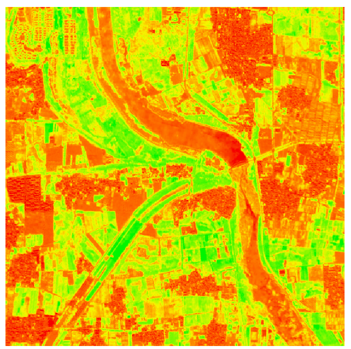
四、可视化实践
# 可视化NDVI
import matplotlib.pyplot as plt

plt.figure(figsize=(12, 8))
plt.imshow(ndvi, cmap='RdYlGn', vmin=-1, vmax=1)
plt.colorbar(label='NDVI')
plt.title('植被指数分布', fontsize=16)
plt.axis('off')
plt.savefig('ndvi_map.png', dpi=300, bbox_inches='tight')
五、实际应用案例
任务:批量处理Landsat8数据提取水体信息
# 示例:批量处理Landsat8数据提取水体信息

# 1. 读取热红外波段
with rasterio.open('landsat8_b10.tif') as src:
    thermal_band = src.read(1)

# 2. 计算地表温度(简单的示例,实际需要进行辐射校正)
temperature = (thermal_band - 273.15)  # 假设热红外波段已经是开尔文温度

# 3. 应用阈值分割提取水体(基于温度或植被指数)
water_mask = temperature < 20  # 假设温度低于20°C为水体

# 4. 输出二值化结果
with rasterio.open('water_mask.tif', 'w', **src.profile) as dst:
    dst.write(water_mask.astype(rasterio.uint8), 1)

# 5. 生成统计报告
import numpy as np
water_area = np.sum(water_mask) * src.res[0] * src.res[1]  # 计算水体面积
print(f'水体面积: {water_area} 平方米')
六、高级功能
- 多线程处理:通过
rasterio.Env()配置GDAL线程数
from rasterio import Env

with Env(GDAL_NUM_THREADS=4):
    with rasterio.open('large_image.tif') as src:
        data = src.read()
- 内存文件操作:使用
MemoryFile处理临时数据 - 数据集拼接:利用
rasterio.merge.merge()实现影像镶嵌 - 分块处理:支持大数据分块读取(chunked reading)
结语
rasterio凭借其简洁的API和强大的功能,已成为遥感数据处理的必备工具。如果你在使用过程中遇到有趣的问题,或者有更好的使用技巧,欢迎在评论区与我们分享!
下期预告
我们将深入探讨如何结合Xarray进行多维遥感数据分析,敬请期待!