当前位置：首页 > news >正文

精通特征选择：过滤器方法提升机器学习模型的技巧

news 来源：原创 2025/5/7 6:47:34

背景

特征选择的定义

特征选择是从数据集中筛选出与目标变量最相关的特征子集的过程。其核心目标是降低数据维度、提升模型性能，并增强结果的可解释性。通过保留关键特征并剔除冗余或无关特征，特征选择能有效加速模型训练、减少过拟合风险，并简化模型结构。

为何需要特征选择？

降低时间和空间复杂度
影响：高维数据会显著增加模型训练的运算量和内存消耗。
原理：通过筛选高价值特征，减少数据处理量和参数计算量。
案例：在垃圾邮件分类任务中，原始特征可能包含发件人、主题关键词、邮件正文等1000多个维度，通过选择前20个关键特征（如“免费领取”“限时折扣”等关键词），训练时间可从数小时缩短至几分钟。
避免“垃圾进，垃圾出”陷阱
影响：无关特征会引入噪声，干扰模型对核心规律的捕捉。
原理：低质量特征导致模型学习到错误模式。
案例：若房屋价格预测模型中混入“房屋外墙颜色”等无关特征，模型可能因噪声数据而错误拟合，预测准确率下降。
遵循简约性原则
影响：简单模型的泛化能力通常优于复杂模型。
原理：奥卡姆剃刀定律指出，在同等解释力下，简单的模型更可能正确。
案例：医疗诊断模型中，仅保留“体温”“白细胞计数”“症状关键词”等关键特征，相比引入数十项检验指标，模型更易验证且误诊率更低。
消除无关特征干扰
影响：冗余特征会稀释重要特征的贡献度。
原理：无关特征对目标变量无统计关联，却占用模型学习资源。
案例：信用卡欺诈检测模型中，“用户昵称”等特征与欺诈行为无关，删除后可提升对“交易金额异常”“跨国IP登录”等关键特征的识别灵敏度。
规避性能退化风险
影响：冗余特征可能导致模型过拟合或欠拟合。
原理：特征过多时，模型可能记忆噪声或忽略关键模式。
案例：图像分类任务中，若保留大量低分辨率像素特征，CNN模型可能在局部噪声中过拟合，而忽略整体纹理特征。
解决多重共线性问题
影响：高度相关的特征会破坏模型稳定性。
原理：共线性特征使参数估计误差增大，导致模型解释性下降。
案例：在房价预测模型中，“房屋面积（平方米）”与“房间数量”存在强相关性。若同时保留，回归模型可能出现系数方向矛盾（如面积越大反而预测价格越低），移除其一后模型更稳定。

过滤方法（Filter Methods）

过滤方法是特征选择的初步筛选手段，通过统计分析特征与目标变量之间的关系或特征本身的统计特性，独立于机器学习模型进行快速筛选。它们使用相关系数、卡方检验或互信息等度量来对特征进行排序，并移除那些未达到一定阈值的特征。其主要优势是计算效率高，适合高维数据预处理。以下是具体方法的详细补充：

(1) 重复列（Duplicate Columns）

定义
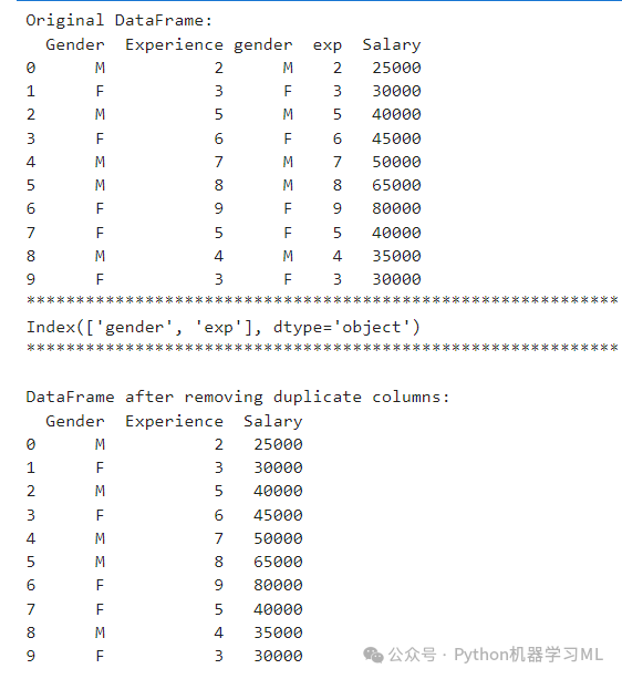
重复列指的是包含相同或非常相似信息的特征。这些重复项不提供任何额外价值，可以删除以简化数据集并提高模型性能。例如，同一数据源可能因采集或存储错误导致两列内容完全重复。

# Import required librariesimport pandas as pd
# Create a DataFrame with duplicate columnsdf = pd.DataFrame({    "Gender": ["M", "F", "M", "F", "M", "M", "F", "F", "M", "F"],    "Experience": [2, 3, 5, 6, 7, 8, 9, 5, 4, 3],    "gender": ["M", "F", "M", "F", "M", "M", "F", "F", "M", "F"],  # Duplicate of "Gender"    "exp": [2, 3, 5, 6, 7, 8, 9, 5, 4, 3],  # Duplicate of "Experience"    "Salary": [25000, 30000, 40000, 45000, 50000, 65000, 80000, 40000, 35000, 30000]})
# Display the original DataFrameprint("Original DataFrame:")print(df)print("*"*60)
# Identify duplicate columnsduplicate_columns = df.columns[df.T.duplicated()]print(duplicate_columns)print("*"*60)
# Drop the duplicate columnscolumns=df.T[df.T.duplicated()].Tdf.drop(columns,axis=1,inplace=True)
# Display the DataFrame after removing duplicate columnsprint("\nDataFrame after removing duplicate columns:")print(df)

(2) 零/低方差特征（Zero/Low Variance Features）

定义

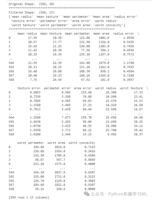
移除方差趋近于零的特征。在数据中变化很小或没有变化的特征，这些特征无法帮助区分结果，因此可以删除以简化模型。

from sklearn.datasets import load_breast_cancerfrom sklearn.feature_selection import VarianceThresholdimport pandas as pd
# Load the Breast Cancer datasetX, y = load_breast_cancer(return_X_y=True, as_frame=True)
# Display the shape of the original feature setprint("Original Shape: ", X.shape)print("*" * 60)
# Initialize VarianceThreshold with a threshold of 0.03# This will filter out features with variance below 0.03vth = VarianceThreshold(threshold=0.03)
# Fit the VarianceThreshold and transform the data# This removes features with low varianceX_filtered = vth.fit_transform(X)
# Display the shape of the filtered feature setprint("Filtered Shape: ", X_filtered.shape)
# Display feature names after filtering# Note: VarianceThreshold does not have get_feature_names_out() method# The following line may not work and could be omitted or replaced with manual feature namesprint(vth.get_feature_names_out())print("*" * 60)
# Create a DataFrame with the filtered features# Feature names might not be available, so using generic names insteadX_filtered_df = pd.DataFrame(X_filtered, columns=vth.get_feature_names_out())
# Display the filtered DataFrameprint(X_filtered_df)

(3)关系

关系在过滤器方法中帮助根据其与目标变量的关系识别最相关的特征。根据涉及的特征类型（分类或数值）使用不同的方法。

1 分类与分类：卡方检验

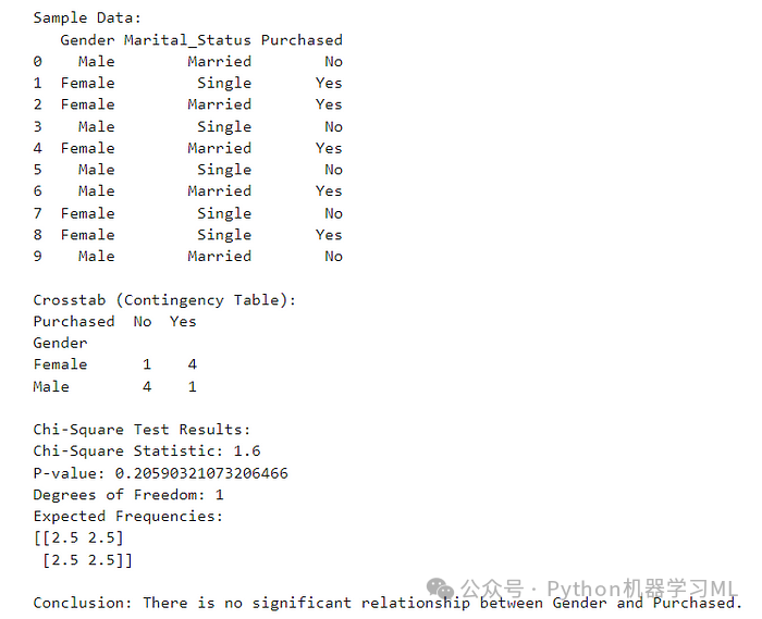
定义：卡方检验通过比较列联表中观察到的和预期的频率来衡量两个分类变量之间的关联。它评估分类变量的分布是否与随机期望的不同。

何时使用：当特征和目标变量都是分类变量时，使用卡方检验。

import pandas as pdfrom scipy.stats import chi2_contingency
# Sample datasetdata = {    'Gender': ['Male', 'Female', 'Female', 'Male', 'Female', 'Male', 'Male', 'Female', 'Female', 'Male'],    'Marital_Status': ['Married', 'Single', 'Married', 'Single', 'Married', 'Single', 'Married', 'Single', 'Single', 'Married'],    'Purchased': ['No', 'Yes', 'Yes', 'No', 'Yes', 'No', 'Yes', 'No', 'Yes', 'No']}
df = pd.DataFrame(data)print("Sample Data:")print(df)
# Create crosstab between Gender and Purchasedcrosstab = pd.crosstab(df['Gender'], df['Purchased'])print("\nCrosstab (Contingency Table):")print(crosstab)
# Perform Chi-Square testchi2, p, dof, expected = chi2_contingency(crosstab)
print("\nChi-Square Test Results:")print(f"Chi-Square Statistic: {chi2}")print(f"P-value: {p}")print(f"Degrees of Freedom: {dof}")print("Expected Frequencies:")print(expected)
# Interpretationif p < 0.05:    print("\nConclusion: There is a significant relationship between Gender and Purchased.")else:    print("\nConclusion: There is no significant relationship between Gender and Purchased.")

2. 分类与数值：方差分析（ANOVA）

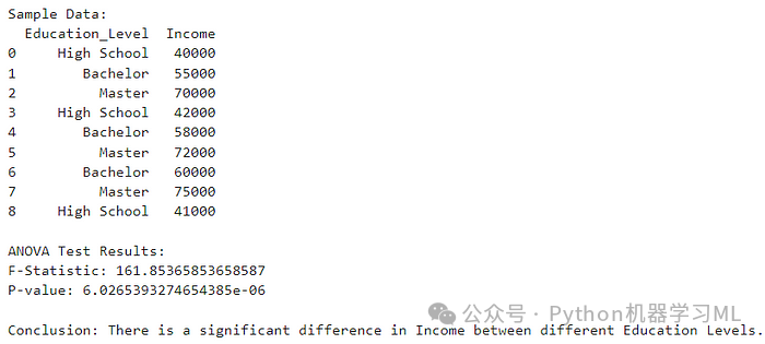
定义：方差分析测试不同组（类别）的数值特征的均值是否有显著差异。它有助于确定分类特征是否对数值目标变量有显著影响。

何时使用：当特征是分类的且目标变量是数值时，使用方差分析。

import pandas as pdfrom scipy.stats import f_oneway
# Sample datasetdata = {    'Education_Level': ['High School', 'Bachelor', 'Master', 'High School', 'Bachelor', 'Master', 'Bachelor', 'Master', 'High School'],    'Income': [40000, 55000, 70000, 42000, 58000, 72000, 60000, 75000, 41000]}
df = pd.DataFrame(data)print("Sample Data:")print(df)
# Group the data by 'Education_Level'groups = df.groupby('Education_Level')['Income'].apply(list)
# Perform ANOVAf_statistic, p_value = f_oneway(*groups)
print("\nANOVA Test Results:")print(f"F-Statistic: {f_statistic}")print(f"P-value: {p_value}")
# Interpretationif p_value < 0.05:    print("\nConclusion: There is a significant difference in Income between different Education Levels.")else:    print("\nConclusion: There is no significant difference in Income between different Education Levels.")

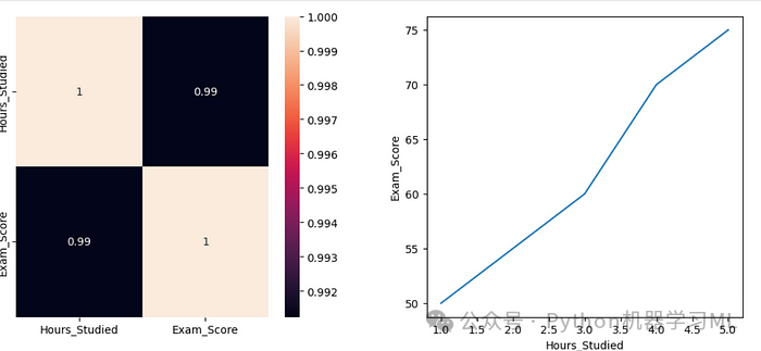
3. 数值与数值：皮尔逊相关系数

定义：皮尔逊相关系数衡量两个数值变量之间的线性关系。其范围从-1（完美的负线性关系）到+1（完美的正线性关系）。

何时使用：当特征和目标变量都是数值时，使用皮尔逊相关系数。

import pandas as pdimport seaborn as snsimport matplotlib.pyplot as plt
# Sample datadata = {'Hours_Studied': [1, 2, 3, 4, 5],        'Exam_Score': [50, 55, 60, 70, 75]}df = pd.DataFrame(data)fig, axes = plt.subplots(1, 2, figsize=(12,5))plt.subplots_adjust(hspace=0.3, wspace=0.3)
# Pearson Correlationcorrelation = df.corr(method="pearson")sns.heatmap(correlation,annot=True,ax=axes[0])sns.lineplot(x=df["Hours_Studied"],y=df["Exam_Score"],ax=axes[1])

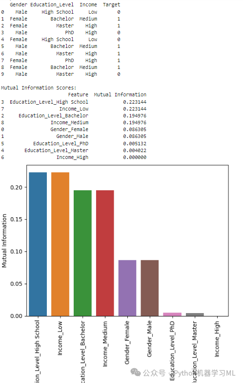
4. 互信息

定义：互信息（MI）衡量一个变量提供关于另一个变量的信息量。它是非线性和非参数的，这意味着它可以捕捉变量之间的任何类型的依赖关系，而不仅仅是线性关系。

高 MI：表示知道一个变量的值可以提供关于另一个变量的重要信息。

低 MI：表示知道一个变量的值对另一个变量的信息量很小。

import pandas as pdfrom sklearn.feature_selection import mutual_info_classiffrom sklearn.preprocessing import OneHotEncoder
# Sample datasetdata = {    'Gender': ['Male', 'Female', 'Female', 'Male', 'Female', 'Male', 'Male', 'Female', 'Female', 'Male'],    'Education_Level': ['High School', 'Bachelor', 'Master', 'PhD', 'High School', 'Bachelor', 'Master', 'PhD', 'Bachelor', 'Master'],    'Income': ['Low', 'Medium', 'High', 'High', 'Low', 'Medium', 'High', 'High', 'Medium', 'High'],    'Target': [0, 1, 1, 0, 0, 1, 1, 1, 1, 0]}
df = pd.DataFrame(data)print("Sample Data:")print(df)
# OneHotEncode categorical featuresencoder = OneHotEncoder(sparse_output=False)encoded_features = encoder.fit_transform(df[['Gender', 'Education_Level', 'Income']])
# Convert the encoded features into a DataFrameencoded_df = pd.DataFrame(encoded_features, columns=encoder.get_feature_names_out())
# Calculate mutual informationmi_scores = mutual_info_classif(encoded_df, df['Target'], discrete_features=True)
# Create a DataFrame to display the MI scoresmi_df = pd.DataFrame({'Feature': encoded_df.columns, 'Mutual Information': mi_scores})mi_df = mi_df.sort_values(by='Mutual Information', ascending=False)print("\nMutual Information Scores:")sns.barplot(x=mi_df["Feature"],y=mi_df["Mutual Information"],hue=mi_df["Feature"])plt.xticks(rotation=90)print(mi_df)

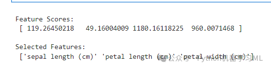
5. 选择最佳 K 个

SelectKBest 是 scikit-learn 中的一种特征选择方法，根据评分函数选择前 k 个特征。它是过滤方法家族的一部分，意味着它独立于模型评估每个特征。

它如何工作

选择评分函数： SelectKBest 需要一个评分函数来对特征进行排序。常见选项包括：

f_classif:ANOVA F 值表示分类任务中标签/特征的 F 值。

chi2: 卡方检验用于独立性。

mutual_info_classif:分类的互信息。

选择最佳特征：根据评分函数，对所有特征进行排名并选择前 k 个特征。

import pandas as pdimport numpy as npfrom sklearn.datasets import load_irisfrom sklearn.feature_selection import SelectKBest, f_classiffrom sklearn.model_selection import train_test_splitfrom sklearn.ensemble import RandomForestClassifierfrom sklearn.metrics import accuracy_score
# 1. Load Datadata = load_iris()X = data.datay = data.target
# Convert to DataFrame for better visualizationdf = pd.DataFrame(X, columns=data.feature_names)df['target'] = y

# 2. SelectKBest# We use the ANOVA F-value as the scoring function for classification tasks.selector = SelectKBest(score_func=f_classif, k=3)  # Select the top 3featuresX_new = selector.fit_transform(X, y)
# Display the scores and selected featuresscores = selector.scores_selected_features = np.array(data.feature_names)[selector.get_support()]print("\nFeature Scores:\n", scores)print("\nSelected Features:\n", selected_features)
# 3. Train-Test SplitX_train, X_test, y_train, y_test = train_test_split(X_new, y, test_size=0.2, random_state=42)
# 4. Train a Modelmodel = RandomForestClassifier()model.fit(X_train, y_train)
# 5. Evaluate the Modely_pred = model.predict(X_test)accuracy = accuracy_score(y_test, y_pred)print("\nModel Accuracy with Selected Features:", accuracy)

过滤方法（Filter Methods）的优缺点

优势

简洁与速度
- 解释
  ：过滤方法基于统计检验快速筛选特征，无需复杂模型训练流程，实现简单且计算效率高。例如，计算方差、相关性或统计检验（如卡方检验）的时间复杂度通常为 (O(n)) 或 (O(n^2))，远低于模型训练的开销。
- 适用场景
  ：高维数据（如文本、基因组数据）的初步降维。
模型独立性
- 解释
  ：通过统计指标（如方差、互信息、相关性）评估特征重要性，方法通用性强，不依赖后续具体模型（如线性回归、随机森林）。
- 适用场景
  ：需快速适配多种模型（如分类和回归任务）的特征选择。
降低过拟合风险
- 解释
  ：过滤方法仅基于统计学规律筛选特征，未使用模型在训练数据上的表现，因此不会学习到数据噪声或随机波动，泛化性更强。
- 适用场景
  ：小样本数据集或噪声较多时，避免模型过早过拟合。

劣势

忽略特征交互
- 解释
  ：过滤方法独立评估单一特征与目标的关系，可能遗漏“联合有效”但“单独无效”的特征组合（例如，特征 A 和 B 需同时存在才能有效预测目标）。
- 案例
  ：在图像识别中，“颜色特征”单独无用，但与“纹理特征”组合时可能显著提升分类性能。
- 影响
  ：对需要特征交互的复杂模型（如神经网络、梯度提升树）效果受限。
可能保留冗余特征
- 解释
  ：过滤方法可能选择与目标相关但彼此高度相关的特征（如“年龄”和“工龄”），导致冗余特征进入模型，增加计算成本且降低可解释性。
- 案例
  ：在金融风控中，若同时保留“月收入”和“年收入”，模型可能重复捕获相似信息。
- 缓解方法
  ：结合相关性分析（如热力图）剔除冗余特征。
依赖先验阈值设定
- 解释
  ：过滤方法需预先设定统计指标阈值（如方差阈值、相关性阈值）。若阈值不合理，可能误删重要特征或保留无用特征。
- 案例
  ：在文本分类中，若方差阈值过高，可能误删稀疏但关键的词频特征。