lesson01-PyTorch初见(理论+代码实战)
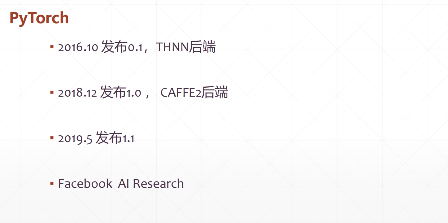
一、初识PyTorch
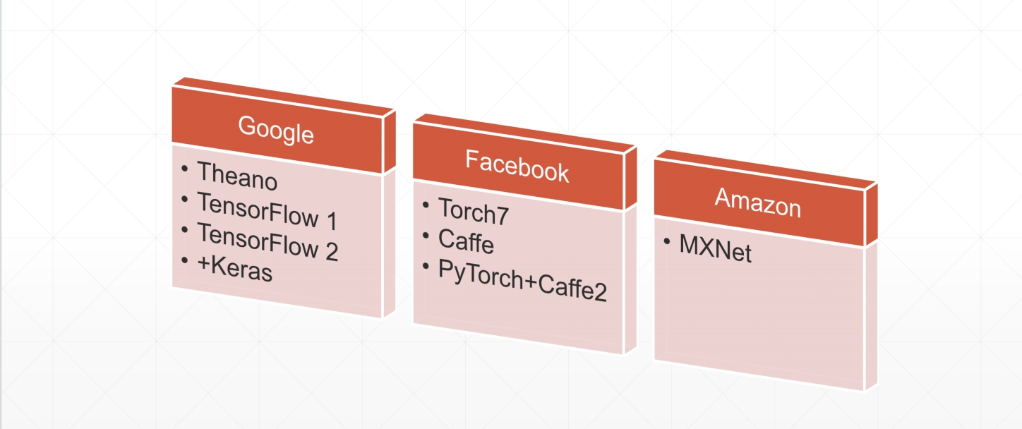
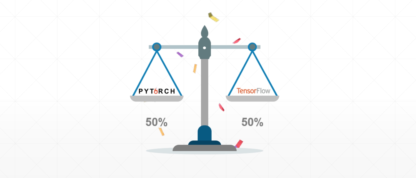
二、同类框架

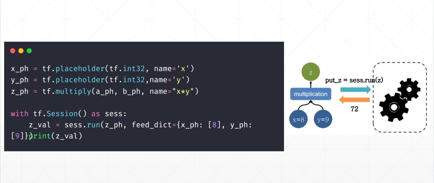
PyTorchVSTensorFlow
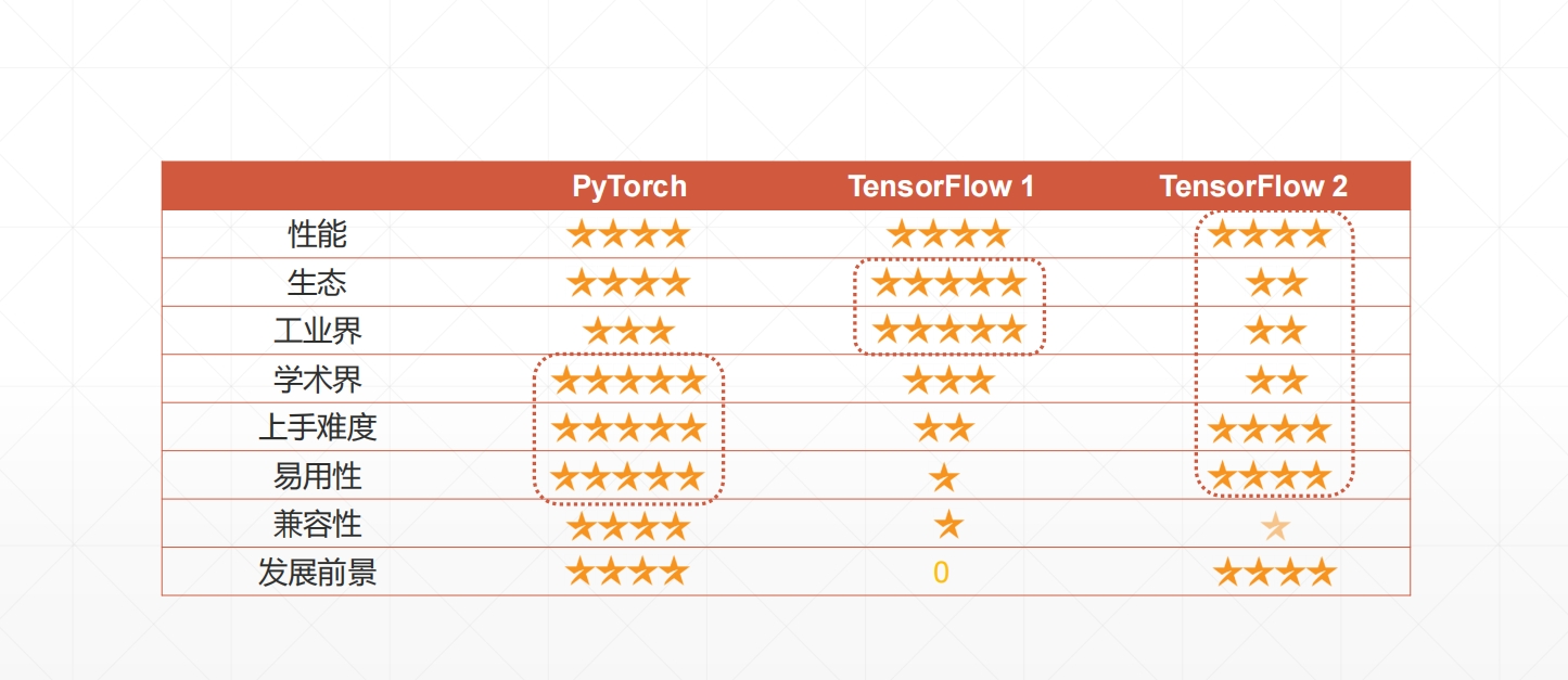
三、参数 对比
四、PyTorch生态

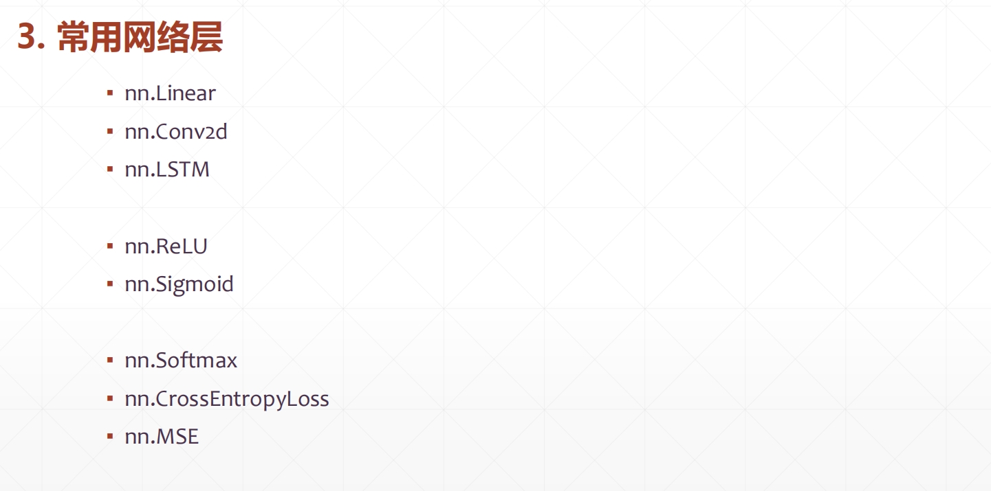
四、常用的网络层
五、代码分析
import torch
from torch import autogradx = torch.tensor(1.)
a = torch.tensor(1., requires_grad=True)
b = torch.tensor(2., requires_grad=True)
c = torch.tensor(3., requires_grad=True)y = a**2 * x + b * x + c
x是一个标量,值为 1.0,不需要梯度。a,b,c都是需要梯度的标量。- 函数
y定义为:
y=a2⋅x+b⋅x+cy=a2⋅x+b⋅x+c
代入当前值:
- a=1
- b=2
- c=3
- x=1
所以:
y=12⋅1+2⋅1+3=1+2+3=6y=12⋅1+2⋅1+3=1+2+3=6
梯度计算部分:
print('before:', a.grad, b.grad, c.grad)
grads = autograd.grad(y, [a, b, c])
print('after :', grads[0], grads[1], grads[2])
初始梯度状态(before):
由于还没有进行反向传播,所有 .grad 属性都是 None。
输出会是:
before: None None None计算梯度(autograd.grad):
我们对函数 y=a2⋅x+b⋅x+cy=a2⋅x+b⋅x+c 分别对 a, b, c 求导:
- ∂a/∂y=2a⋅x=2⋅1⋅1=2
- ∂y/∂b=x=1
- ∂y/∂c=1
所以梯度应该是:
grads[0] = 2grads[1] = 1grads[2] = 1
最终输出示例:
before: None None None
after : tensor(2.) tensor(1.) tensor(1.)- 这段代码演示了如何使用
torch.autograd.grad来手动计算多个变量对某个标量输出的梯度。
代码案例二
import 	torch
import  time
print(torch.__version__)
print(torch.cuda.is_available())
# print('hello, world.')a = torch.randn(10000, 1000)
b = torch.randn(1000, 2000)t0 = time.time()
c = torch.matmul(a, b)
t1 = time.time()
print(a.device, t1 - t0, c.norm(2))device = torch.device('cuda')
a = a.to(device)
b = b.to(device)t0 = time.time()
c = torch.matmul(a, b)
t2 = time.time()
print(a.device, t2 - t0, c.norm(2))t0 = time.time()
c = torch.matmul(a, b)
t2 = time.time()
print(a.device, t2 - t0, c.norm(2))
代码解析
1. 导入模块与基本信息打印
import torch
import timeprint(torch.__version__)
print(torch.cuda.is_available())torch.__version__:输出当前安装的 PyTorch 版本。torch.cuda.is_available():判断当前是否可用 CUDA(即是否有支持的 GPU)。
示例输出:
2.4.0
True
2. 定义两个大张量用于矩阵乘法
a = torch.randn(10000, 1000)
b = torch.randn(1000, 2000)a是一个形状为(10000, 1000)的随机张量(正态分布)。b是一个形状为(1000, 2000)的随机张量。- 矩阵乘法后,结果
c的形状将是(10000, 2000)。
3. 在 CPU 上进行矩阵乘法并计时
t0 = time.time()
c = torch.matmul(a, b)
t1 = time.time()
print(a.device, t1 - t0, c.norm(2))- 使用
torch.matmul(a, b)计算矩阵乘法。 a.device显示设备信息,默认是'cpu'。t1 - t0是计算时间差(单位秒)。c.norm(2)是为了防止编译器优化掉无输出的运算,同时验证结果的一致性。
4. 将张量移到 GPU 上
device = torch.device('cuda')
a = a.to(device)
b = b.to(device)
5. 第一次在 GPU 上进行矩阵乘法并计时
t0 = time.time()
c = torch.matmul(a, b)
t2 = time.time()
print(a.device, t2 - t0, c.norm(2))- 这里会受到 GPU 初始化开销 和 CUDA 内核启动延迟 的影响,第一次运行通常较慢。
6. 第二次在 GPU 上进行矩阵乘法并计时
t0 = time.time()
c = torch.matmul(a, b)
t2 = time.time()
print(a.device, t2 - t0, c.norm(2))- 第二次运行没有初始化开销,更能反映真实性能。
预期输出示例(假设你有 GPU)
2.4.0
True
cpu 0.123456 tensor(7070.5678)
cuda:0 0.201234 tensor(7070.5678, device='cuda:0')
cuda:0 0.012345 tensor(7070.5678, device='cuda:0')
✅ 总结分析
| 操作 | 设备 | 时间 (秒) | 备注 |
|---|---|---|---|
| 第一次 matmul | CPU | ~0.12s | 常规速度 |
| 第一次 GPU matmul | GPU | ~0.20s | 包含初始化和首次调用延迟 |
| 第二次 GPU matmul | GPU | ~0.01s | 实际 GPU 加速效果 |
🔍 补充说明
- 为什么第一次 GPU 运行比 CPU 还慢?
- 因为第一次调用涉及 CUDA 内核启动、内存拷贝、上下文初始化等额外开销。
- 第二次 GPU 调用很快:是因为这些准备工作已经完成,真正体现了 GPU 并行计算的优势。
- norm(2):用来确保张量被实际计算,避免因“未使用”而被优化掉。
🛠️ 优化建议
如果你要准确测试 GPU 的性能,可以:
-
预热(Warm-up):先做几次空跑。
for _ in range(5):_ = torch.matmul(a, b)
torch.cuda.synchronize()  # 同步等待完成
使用 torch.cuda.Event 来更精确计时:
start = torch.cuda.Event(enable_timing=True)
end = torch.cuda.Event(enable_timing=True)start.record()
c = torch.matmul(a, b)
end.record()
torch.cuda.synchronize()
print(start.elapsed_time(end))  # 单位是毫秒