网站开发 报价广告推广赚钱在哪接
种一棵树最好的时间是十年前,其次是现在。
目录
前言
一、数据准备
二、构建模型
三、模型精度检验
前言
最近又空闲下来,终于有时间把之前荒废的学习计划给重拾起来了!今天做的是MNIST手写数字识别项目。这可以说是深度学习的“Hello World”级项目了。在AI的帮助下,也是成功的完成了这个项目。记录下来,其中如有不正确的地方,欢迎指正。
一、数据准备
做项目最重要的是什么?数据!因此,我们首先把数据准备好。
我使用的框架是Pytorch,在Pytorch中有现成的方法直接下载。直接通过 torchvision.datasets 模块提供的接口完成。首先需要安装torchvision。
pip install torchvision下载数据,代码如下。运行后会直接下载到data文件夹,如果没有会直接在当前文件路径新建一个。
from torchvision import datasets, transforms# 定义数据预处理(这里仅做归一化,将像素值从 [0,255] 转为 [0,1])
transform = transforms.Compose([transforms.ToTensor(),  # 转为 PyTorch 张量(形状:[1,28,28])transforms.Normalize((0.1307,), (0.3081,))  # MNIST 全局均值和标准差(经验值)
])# 下载训练集(6万张图)
train_dataset = datasets.MNIST(root='./data',  # 数据集存储路径(当前目录下的 data 文件夹)train=True,     # 是否为训练集(True:训练集,False:测试集)download=True,  # 若本地无数据则下载transform=transform  # 应用预处理
)# 下载测试集(1万张图)
test_dataset = datasets.MNIST(root='./data',train=False,download=True,transform=transform
)
当然,如果使用的是tensorflow框架的话,也是有现成的方法,但是tensorflow使用起来要比Pytorch稍微难上手一点。除此之外,也可以选择直接去官方网站下载
下载完后,我们查看数据集大小,以及对各数字类别分布做一个统计,这样做的目的是为了对这个数据集有更多的了解。机器学习非常依赖数据,所以在进行模型训练前,我们应该对数据集有尽可能多的了解。代码及运行结果如下。
from torch.utils.data import DataLoadertrain_loader = DataLoader(train_dataset, batch_size=64, shuffle=True)  # 训练集批量加载(打乱顺序)
test_loader = DataLoader(test_dataset, batch_size=128, shuffle=False)   # 测试集批量加载(不打乱)
# 训练集和测试集的图片数量
print(f"训练集图片数量: {len(train_dataset)} 张")  # 输出:60000 张
print(f"测试集图片数量: {len(test_dataset)} 张")   # 输出:10000 张
import numpy as np# 统计训练集标签分布
train_labels = [label for _, label in train_dataset]
train_label_counts = np.bincount(train_labels)  # 统计0-9每个数字的出现次数# 统计测试集标签分布
test_labels = [label for _, label in test_dataset]
test_label_counts = np.bincount(test_labels)# 绘制柱状图
plt.figure(figsize=(12, 5))# 训练集子图
plt.subplot(1, 2, 1)
plt.bar(range(10), train_label_counts)
plt.title("distribution of categories in train set")
plt.xlabel("label")
plt.ylabel("number")# 测试集子图
plt.subplot(1, 2, 2)
plt.bar(range(10), test_label_counts)
plt.title("distribution of categories in test set")
plt.xlabel("label")
plt.ylabel("number")plt.tight_layout()
plt.show()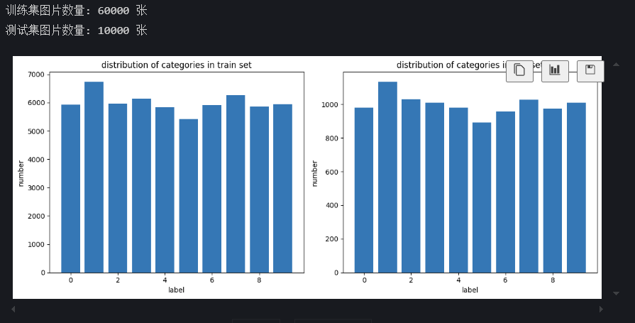
二、构建模型
导入相关库
import torch
import torch.nn as nn
import torch.nn.functional as F
import torch.optim as optim
import matplotlib.pyplot as plt
import numpy as np
import pandas as pd
构建模型,我这里选择搭建了一个三层全连通感知机模型。
class ThreeLayerPerceptron(nn.Module):def __init__(self, input_dim, hidden_dim1, hidden_dim2, output_dim):super(ThreeLayerPerceptron, self).__init__()# 第一层全连接:输入层 -> 隐藏层1self.fc1 = nn.Linear(input_dim, hidden_dim1)# 第二层全连接:隐藏层1 -> 隐藏层2self.fc2 = nn.Linear(hidden_dim1, hidden_dim2)# 第三层全连接:隐藏层2 -> 输出层self.fc3 = nn.Linear(hidden_dim2, output_dim)def forward(self, x):# 输入数据展平(如果是图像等多维输入需要此操作)x = x.view(x.size(0), -1)# 第一层:线性变换 + ReLU激活x = F.relu(self.fc1(x))# 第二层:线性变换 + ReLU激活x = F.relu(self.fc2(x))# 第三层:线性变换(输出层通常不接激活函数,用于分类时后续接softmax)x = self.fc3(x)return x进行模型训练。我们这里是训练了5个epoch,意味着整个数据集经历了五次前向传播和反向传播。其实迭代很少了,但是这个任务比较简单,所以虽然只是经过了简单的训练,但是最后的效果还行。
# 模型参数(以MNIST为例)
input_dim = 784       # 28x28图像展平后的维度
hidden_dim1 = 256     # 第一个隐藏层神经元数
hidden_dim2 = 128     # 第二个隐藏层神经元数
output_dim = 10       # 10类数字# 初始化模型(自动适配CPU/GPU)
device = torch.device("cuda" if torch.cuda.is_available() else "cpu")
model = ThreeLayerPerceptron(input_dim, hidden_dim1, hidden_dim2, output_dim).to(device)# 定义损失函数(分类任务用交叉熵)和优化器(Adam)
criterion = nn.CrossEntropyLoss()
optimizer = optim.Adam(model.parameters(), lr=0.001)
def train_model(model, train_loader, criterion, optimizer, epochs=10):model.train()  # 切换训练模式(启用Dropout等)for epoch in range(epochs):running_loss = 0.0correct = 0total = 0for batch_idx, (images, labels) in enumerate(train_loader):# 数据移动到目标设备(CPU/GPU)images, labels = images.to(device), labels.to(device)# 前向传播 + 计算损失outputs = model(images)loss = criterion(outputs, labels)# 反向传播 + 优化参数optimizer.zero_grad()  # 清空梯度loss.backward()        # 反向传播optimizer.step()       # 更新参数# 统计训练指标running_loss += loss.item()_, predicted = torch.max(outputs.data, 1)  # 取概率最大的类别total += labels.size(0)correct += (predicted == labels).sum().item()# 每100个批量打印一次进度if (batch_idx+1) % 100 == 0:print(f"Epoch [{epoch+1}/{epochs}], Batch [{batch_idx+1}/{len(train_loader)}], "f"Loss: {running_loss/100:.4f}, Acc: {100*correct/total:.2f}%")running_loss = 0.0  # 重置累计损失print("训练完成!")# 开始训练(建议先试3-5轮,观察准确率是否提升)
train_model(model, train_loader, criterion, optimizer, epochs=5)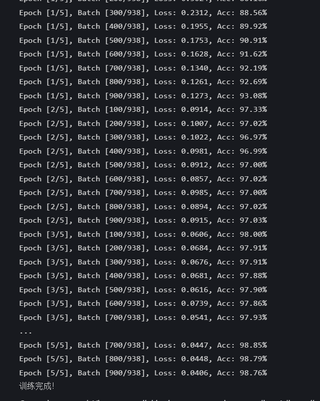
三、模型精度检验
测试集精度验证
ef test_model(model, test_loader):model.eval()  # 切换测试模式(禁用Dropout等)correct = 0total = 0with torch.no_grad():  # 不计算梯度(加速测试)for images, labels in test_loader:images, labels = images.to(device), labels.to(device)outputs = model(images)_, predicted = torch.max(outputs.data, 1)total += labels.size(0)correct += (predicted == labels).sum().item()print(f"测试准确率: {100 * correct / total:.2f}%")# 运行测试
test_model(model, test_loader)
测试集准确率为0.9762,结合之前的训练集准确率为0.9876,可以看到效果还是不错的。
接下来进行混淆矩阵热图可视化。几乎都集中在对角线,模型性能不错。
from sklearn.metrics import confusion_matrix
import seaborn as snsdef plot_confusion_matrix(model, test_loader):model.eval()all_labels = []all_preds = []with torch.no_grad():for images, labels in test_loader:images, labels = images.to(device), labels.to(device)outputs = model(images)_, preds = torch.max(outputs, 1)all_labels.extend(labels.cpu().numpy())all_preds.extend(preds.cpu().numpy())# 计算混淆矩阵cm = confusion_matrix(all_labels, all_preds)# 可视化plt.figure(figsize=(10, 8))sns.heatmap(cm, annot=True, fmt='d', cmap='Blues', xticklabels=range(10), yticklabels=range(10))plt.xlabel('predicted')plt.ylabel('true')plt.title('Confusion Matrix')plt.show()# 调用函数(需已定义model和test_loader)
plot_confusion_matrix(model, test_loader)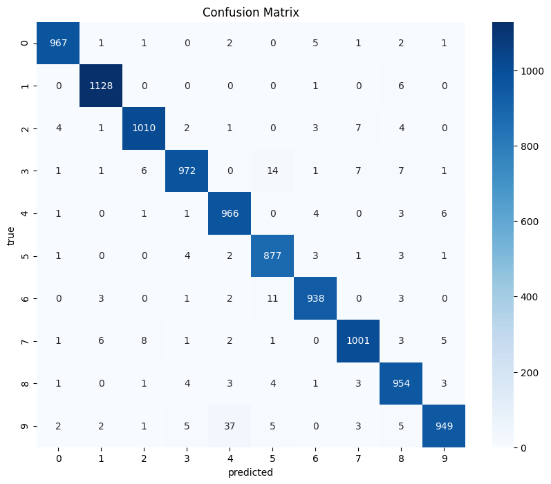
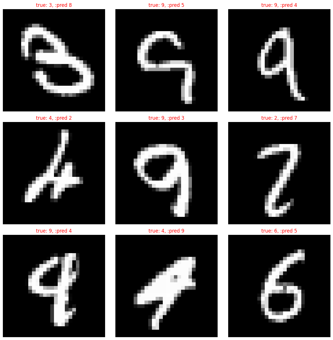
错误样本可视化,展示模型分类错误的样本,分析误分类原因
def plot_wrong_samples(model, test_loader, num_samples=9):model.eval()wrong_images = []wrong_labels = []wrong_preds = []with torch.no_grad():for images, labels in test_loader:images, labels = images.to(device), labels.to(device)outputs = model(images)_, preds = torch.max(outputs, 1)# 筛选错误样本mask = (preds != labels)if mask.any():wrong_images.extend(images[mask].cpu())wrong_labels.extend(labels[mask].cpu().numpy())wrong_preds.extend(preds[mask].cpu().numpy())if len(wrong_images) >= num_samples:break# 可视化前9个错误样本plt.figure(figsize=(12, 12))for i in range(num_samples):image = wrong_images[i].squeeze() # 移除通道维度true_label = wrong_labels[i]pred_label = wrong_preds[i]plt.subplot(3, 3, i+1)plt.imshow(image, cmap='gray')plt.title(f'true: {true_label}, :pred {pred_label}', color='red')plt.axis('off')plt.tight_layout()plt.show()
结果如下:
计算类别级准确率,查看每个类别的分类准确率。
def plot_class_accuracy(model, test_loader):model.eval()class_correct = [0] * 10class_total = [0] * 10with torch.no_grad():for images, labels in test_loader:images, labels = images.to(device), labels.to(device)outputs = model(images)_, preds = torch.max(outputs, 1)for label, pred in zip(labels, preds):if label == pred:class_correct[label] += 1class_total[label] += 1# 计算每个类别的准确率class_acc = [100 * class_correct[i]/class_total[i] for i in range(10)]# 绘制柱状图plt.figure(figsize=(10, 6))plt.bar(range(10), class_acc)plt.xticks(range(10))plt.xlabel('label')plt.ylabel('accuracy(%)')# plt.title('各类别分类准确率')plt.ylim(80, 100)  # MNIST模型通常准确率较高,调整Y轴范围plt.show()# 调用函数
plot_class_accuracy(model, test_loader)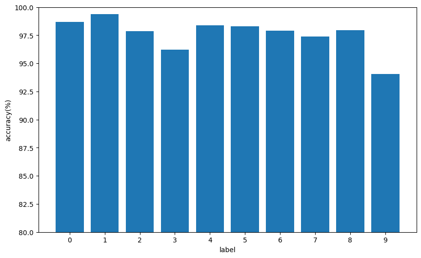
其实从几个样本的结果,还有柱状图,可以看出模型对9这个数字的识别明显不如其他类别。